Quantitative Agricultural Flood Risk Assessment Using Vulnerability Surface and Copula Functions


1
Grassland Research Institute, Chinese Academy of Agricultural Science, Hohhot 010010, China
2
College of Geographical Science, Inner Mongolia Normal University, Hohhot 010022, China
3
Inner Mongolia Key Laboratory of Disaster and Ecological Security on the Mongolian Plateau, Hohhot 010022, China
*
Author to whom correspondence should be addressed.
Water 2018, 10(9), 1229; https://doi.org/10.3390/w10091229
Submission received: 20 July 2018
/
Revised: 29 August 2018
/
Accepted: 1 September 2018
/
Published: 12 September 2018
(This article belongs to the Section Hydrology)
Abstract
:Agricultural flood disaster risk assessment plays a vital role in agricultural flood disaster risk management. Extreme precipitation events are the main causes of flood disasters in the Midwest Jilin province (MJP). Therefore, it is important to analyse the characteristics of extreme precipitation events and assess the flood risk. In this study, the Multifractal Detrended Fluctuation Analysis (MF-DFA) method was used to determine the threshold of extreme precipitation events. The total duration of extreme precipitation and the total extreme precipitation were selected as flood indicators. The copula functions were then used to determine the joint distribution to calculate the bivariate joint return period, which is the flood hazard. Historical data and flood indicators were used to build an agricultural flood disaster vulnerability surface model. Finally, the risk curve for agricultural flood disasters was established to assess the flood risk in the MJP. The results show that the proposed approaches precisely describe the joint distribution of the flood indicators. The results of the vulnerability surface model are in accordance with the spatiotemporal distribution pattern of the agricultural flood disaster loss in this area. The agricultural flood risk of the MJP gradually decreases from east to west. The results provide a firm scientific basis for flood control and drainage plans in the area.
1. Introduction
Floods pose serious threats to the economy and life worldwide, especially to rural inhabitants of developing countries. Floods rank third among all natural disasters based on the degree of severity, extent of influence, yield reduction, casualties, and social effects [1]. The frequency and intensity of floods are expected to increase due to climatic and non-climatic factors, such as the El Niño Southern Oscillation (ENSO), extreme precipitation events, increasing rate of deforestation, and rapid urbanization [2,3,4]. Statistics show that more than 520 million people are affected by disastrous floods and approximately 25,000 deaths occur annually across the world [5]. The worldwide increase in damages caused by floods during the last decades demonstrates that the risk level is significantly increasing [6,7,8].
Floods are natural disasters with a high frequency of occurrence, wide range of hazards, and the most serious impact on people’s survival and development in China [9]. According to statistics from 1972 to 2013, floods annually affect an area up to 1.05 × 10⁵ km2 and lead to 2 × 10⁵ million yuan in annual losses in China [10]. The bulletin of flood and drought disasters in China reported on floods and extreme precipitation, with both showing a synchronous increase since 2008, and the total flood disaster area of the crops associated with extreme precipitation increased from 2006–2013 [11]. This means that the effect of flood disasters is closely related to the intensity of the precipitation, and the extreme precipitation can be used to some extent to analyse the evolution and influence of the flood. The study area is located in the Midwest Jilin province (MJP), which is part of the mollisol region of northeastern China and includes one of the three famous maize belts of the world. However, the MJP is also an area influenced by flood disasters and this often results in yield reduction. In the 1990s, floods occurred almost every three years in the area, with high intensity, wide range, and heavy losses [12]. The most serious one is extensive rainfall, which caused floods in the region in July 2010, and affected tens of thousands of families. It was estimated that the total direct economic loss exceeded 1.03 billion yuan [13]. Therefore, it is important to assess the risk of flood disasters to develop strategies to mitigate flood hazards and reduce losses.
There are two mainstream approaches to assess flood risk. The first approach is probabilistic risk assessment, which is mainly to use the probabilistic method to calculate the probability and consequences of flood disasters in a certain area. For example, the flood risk for a planned detention area along the Elbe River in Germany was assessed based on two loss and probability estimation approaches of different time frames [14]. Xu et al. assessed the flood catastrophe risk for the grain production at the provincial scale in China based on the block maxima model [15]. Sun et al. calculated the agricultural flood risk at Henan Province, China using the information diffusion method (IDM) [16]. It is clear that probabilistic risk assessment is mainly suitable for single-factor analysis. It involves simple calculations; however, the shortcomings are that the risk formation mechanism and influencing factors of flood disasters are not reflected. The other is an agricultural flood risk assessment method based on the risk formation mechanism. It uses the various elements of the disaster risk system to analyse the elements of agricultural flood disaster risk and quantify the risk factors. The risk factors are then combined using certain paradigms. Finally, the agricultural flood risk is defined based on a comprehensive flood disaster risk index. Gain et al. implemented flood risk assessment in the Dhaka City, Bangladesh using an integrated flood risk assessment approach. They not only calculated a valuation of direct tangible costs, but also incorporated the physical dimensions into the hazard and exposure and social dimensions into vulnerability [17]. Duan et al. evaluated and predicted the late rice flood disaster risk degree in the production and growth period and temporal and spatial differences based on the late rice flood disaster risk assessment model [18]. Ghosh and Kar applied an analytical hierarchy process (AHP) for flood risk assessment in Malda district of West Bengal, India through incorporating flood hazard elements and vulnerability indicators in a geographical information system environment [19]. Based on the standard formulation of natural disaster risk, Guo et al. combined flood risk factors of hazard, exposure, vulnerability, and restorability, and assessed the integrated flood risk in central Liaoning Province, China [20]. Moreover, related research on single risk factors has also received much attention. Derdous et al. presented an approach to predict and assess downstream hazards associated with dam break flooding by the integration of hydraulic modelling and geographic information system (GIS) [21]. Luu et al. analysed flood hazard using flood mark data, including flood depth and flood duration [22]. Based on the combining of exposure, sensitivity, and adaptability, Wu et al. assessed agricultural vulnerability to floods by using emergy and a landscape fragmentation index [23]. Paprotny et al. utilized a gridded reconstruction of flood exposure in 37 European countries and a new database of damaging floods since 1870 [24]. Nevertheless, the assessment using the above methods has some limitations: First, the process of indicator selection may be biased; second, it requires a significant amount of data for the calculation; and third, it does not adequately reflect the connection between the flood risk factors.
The vulnerability curve is used to express the loss rate of crops under different disaster intensities in a table or curve form, which indicates the intrinsic relationship between the intensity of the disaster-causing factor and the vulnerability of the hazard-affected body [25]. However, most of the existing results are flood vulnerability curves constructed from single-hazard and disaster loss data [26,27]. The correlation between multi-hazard and loss data is not much expressed. Therefore, considering the connection between extreme precipitation events and floods [28,29], multifractal detrended fluctuation analysis (MF-DFA) was used to define the threshold of extreme precipitation events as the hazard factor and the copula function was applied to calculate the joint return period in this study. The vulnerability surface, a model that can be used to calculate vulnerability to multi-hazards [30], was considered in this paper to express the flood vulnerability. Finally, a quantitative agricultural flood risk assessment method was proposed, which integrates the vulnerability surface and the joint return period, providing new ideas for flood risk assessment research. Overall, the objective of this study was to extend univariate to multivariate risk assessment within the copula framework in MJP. Meanwhile, the flood loss can be evaluated using the different return periods. The results promote a better understanding of the local history of flood disasters and their social impact, and provide the local government with a strong scientific basis for flood control and drainage plans.
2. Materials and Methods
2.1. Study Region
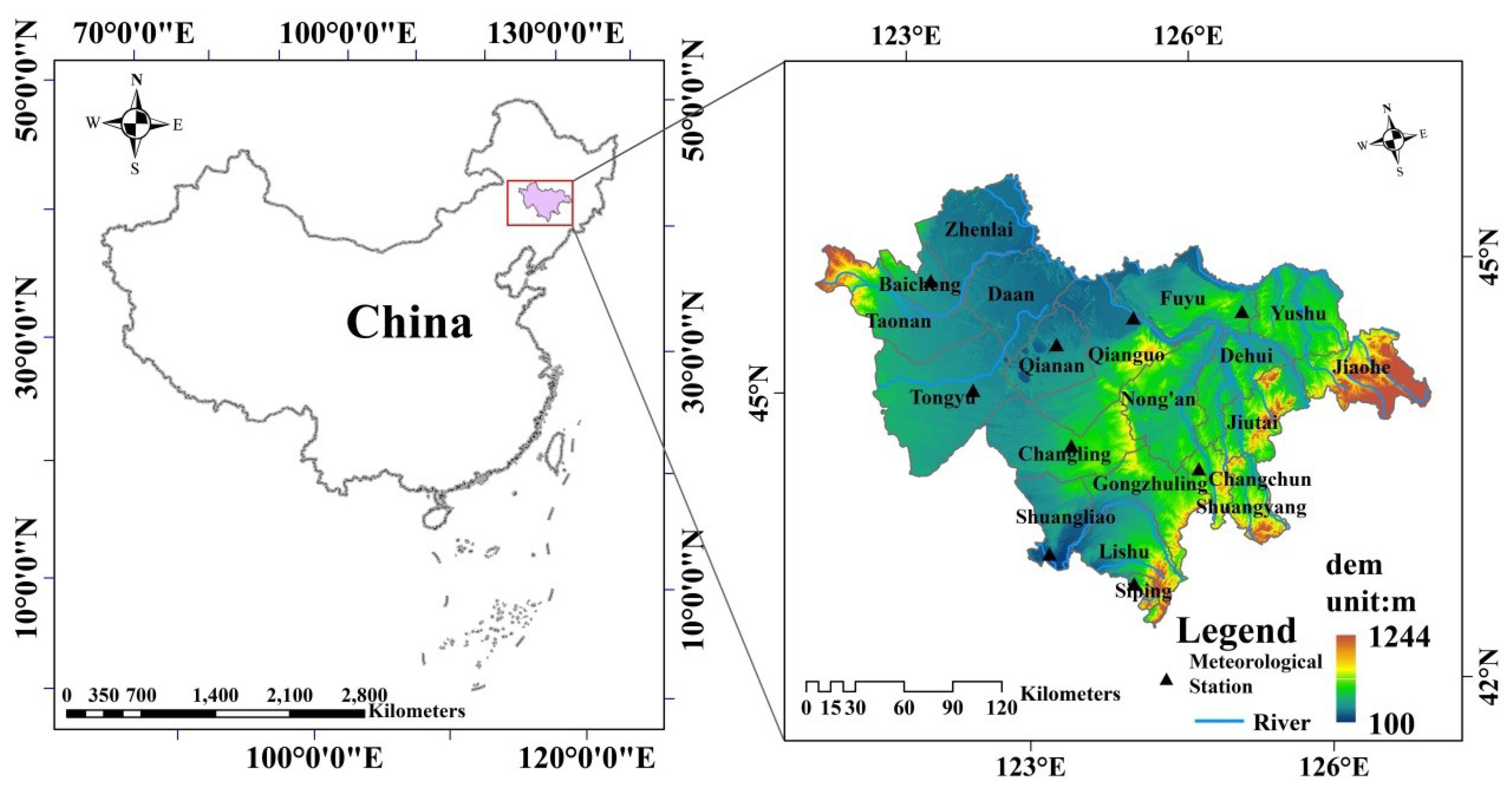
The Midwest Jilin Province is located in Northeast China between 43°16′ N–46°18′ N and 121°38′ E–127°45′ E. It is administratively divided into five cities (Figure 1): Baicheng, Songyuan, Siping, Changchun, and Jilin. The study area is in the temperate subhumid and semi-arid zones. The average temperature varies by 4.9 °C to 5.5 °C. The temperatures reach a maxima of 34.8 °C–39.5 °C in July, while the minima temperatures range from −38 °C to −39.8 °C in January. The sunshine time varies from 2630 to 2930 h, and the relative humidity ranges from 52% to 61%. The average precipitation varies from 399.7 to 576.7 mm, and mainly occurs from June to September, occupying 60–80% of the annual precipitation. The evaporation ranges from 1638.9 to 1833.4 mm. The moist forest ecosystem transitions to semi-arid steppe and arid desert belt; it is sensitive to environmental changes.
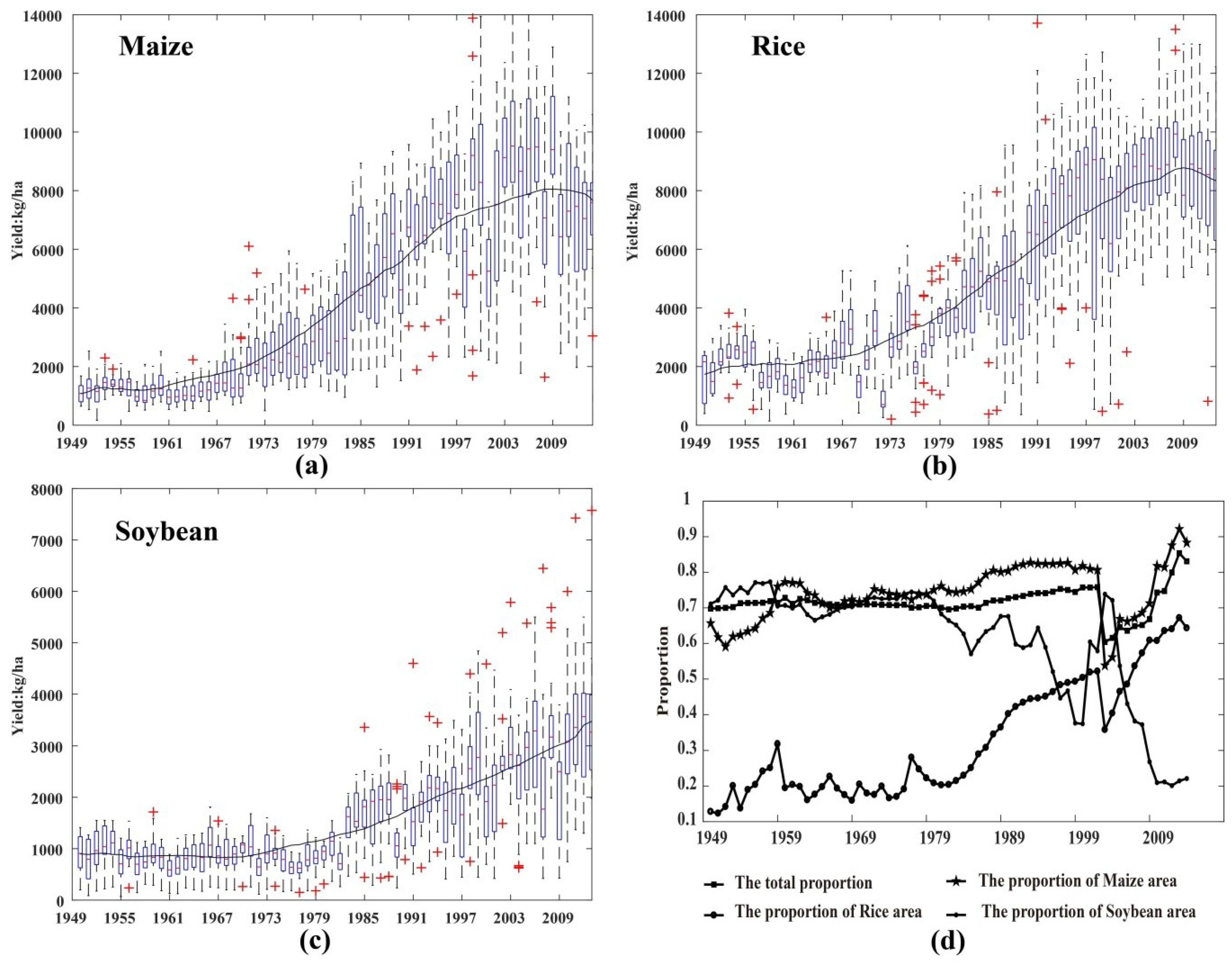
The total area of the MJP is 8.29 × 10⁴ km2, accounting for 44.23% of the Jilin Province. The MJP is one of the main distribution areas of black soil and maize in China. The so-called golden maize zone has a good reputation because of the good quality, properties, and starch content [31]. The total cereal and oilseeds area is 4.79 × 10⁶ ha, which accounts for 83.10% of the total area. Crops include maize, rice, potatoes, soybeans, sunflower seeds, fruits, tobacco, and beet. The main types of crops are maize, rice, and soybeans. The proportions of these individual crops of the planted area in the MJP in 2014 were as follows: 71.01%, 11.07%, and 4.20%, respectively [32]. In addition to soybeans, the acreage of maize and rice volatility is increasing. The yield of maize and rice has been declining in recent years due to the occurrence of disastrous weather. On the contrary, the total area of grain and oil crops is increasing. The maize and soybean yields are increasing at a rate of 13.56 kg/ha and 3.8 kg/ha per ten years, respectively (Figure 2).
2.2. Data Source and Processing
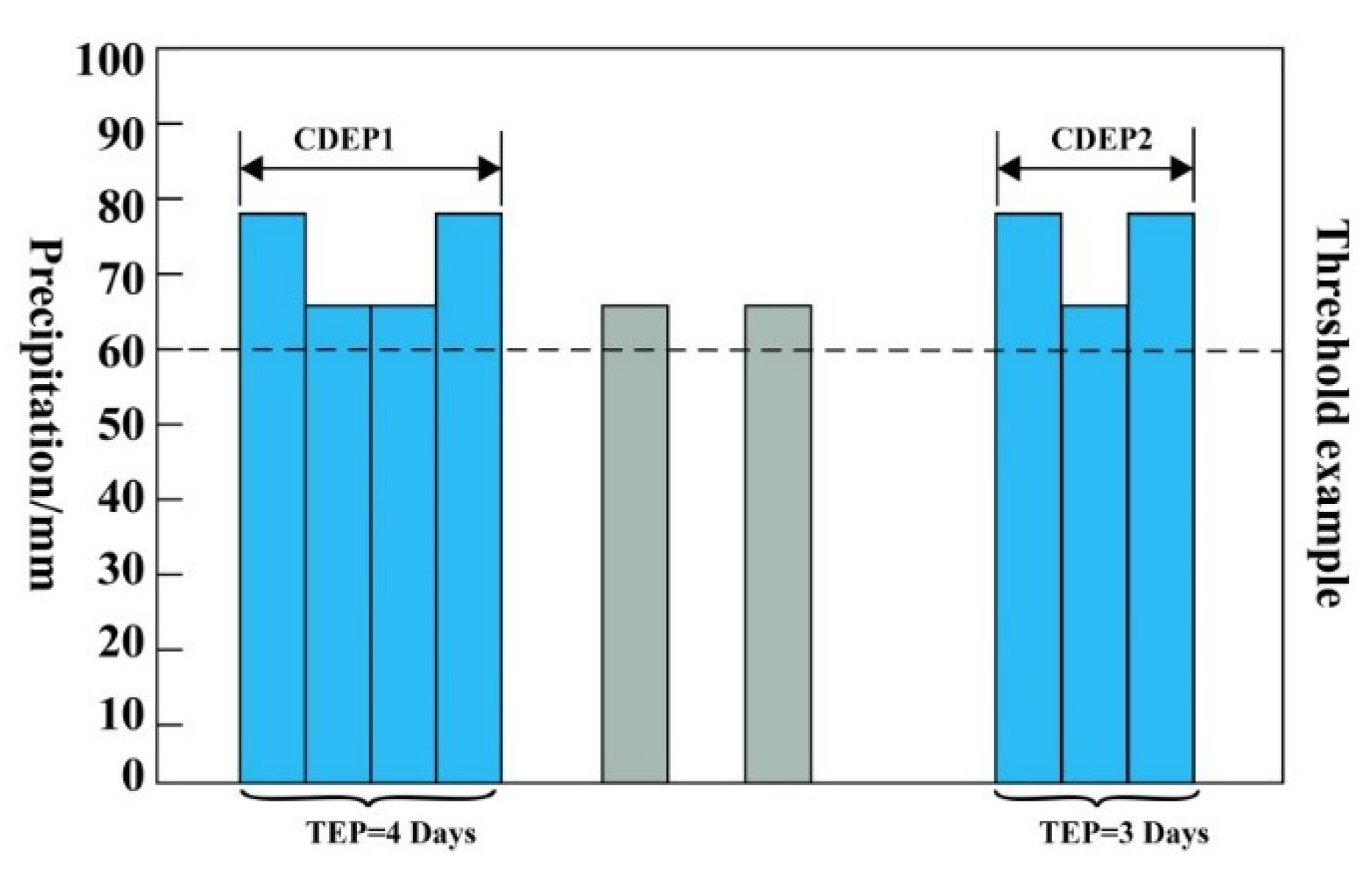
Daily precipitation data of nine stations from 1960 to 2014 were collected from the China Meteorological Data Network. The data of crop production loss caused by flood disasters were derived from the Chinese meteorological disasters ceremony [33] and the Yearbook of Chinese urban disasters and China agricultural meteorology disaster situation datasets, and cover 55 years between 1960–2014. The total extreme precipitation (TEP) and the number of consecutive days with precipitation ≥0.1 mm during extreme precipitation events (CDEP) were selected in this study as the two flood indicators stipulating the intensity and duration of the flood, respectively (Figure 3). The agricultural flood loss was obtained from the affected area of the crops showing a yield reduction of more than 10% of the crop planting area caused by flood disasters.
2.2.1. Multifractal Detrended Fluctuation Analysis Method
The Multifractal Detrended Fluctuation Analysis (MF-DFA) proposed by Kantelhardt can detect the long-range correlation of time series, define its fractal structure, determine whether the time series has multi-fractal features, and determine its multi-fractal characteristics [34]. In recent years, it has been widely applied in the studies of extreme climate events [35,36,37]. The DFA index defines the system evolution of long-range correlation in a certain period. Extreme events do not (or are small) affect the long-range correlation of the entire system [34]. The DFA index, therefore, determines the threshold of the extreme events. This method was employed in our study to characterize the extreme precipitation events.
2.2.2. Marginal Distribution Functions
The flood disaster indicators are random variables and the distributions affecting the two variables are unknown. Hence, we assume that the two indicators obey a certain distribution. The statistical parameters were calculated based on this hypothesis. The determination of the distribution parameters is crucial because they affect the reliability. In this study, we use the normal distribution (NORM), Poisson distribution (POISS), exponential distribution (EXP), extreme value distribution (EV), generalized extreme value distribution (GEV), generalized Pareto distribution (GP), and Gamma distribution (GAM) to fit the flood disaster indicators [38]. Additionally, the maximum likelihood function was applied to estimate the marginal distribution parameters:
where, is the likelihood function, is the marginal distribution density function, and are the estimated parameters. The goodness of the marginal distribution fit was calculated using the Kolmogorov-Smirnov test (K-S) to choose the optimal probability distribution function for the two flood disaster variables.
2.2.3. Joint Distribution Function of the Flood Indicators
The joint distribution function of flood indicators is established by using the marginal distribution function and related structure. We chose three types of Archimedean copula functions to calculate the joint distribution of the flood indicators from the existing Copula function [39]. The specific joint distribution function and space of the parameters are shown in Table 1.
We can use the copula function to fit the bivariate joint distribution and determine the optimal copula joint function that meets the parameter range using the root mean square error (RMSE) and the Akaike information criterion (AIC). The equation is as follows:
where Pei denotes the bivariate joint empirical probability of the extreme precipitation factors, Pi is the probability of the copula joint distribution function, and i represents the number of parameters in the model.
2.2.4. Joint Return Period of Flood Indicators
The return period theory indicates that the return period of certain elements in extreme precipitation events is greater than or equal to a specific value:
where, represents the univariate return period of extreme precipitation indicators while indicates the marginal distribution of each indicator. N is the duration (year) of sample observation, and n is the number of occurrences beyond a given sample in the observation period [40,41]. The bivariate joint return period for the copula joint function is expressed as:
2.2.5. The Vulnerability Surface Model
The vulnerability surface was generated using trend surface analysis, which simulates the spatial distribution and variation of the geographical elements [42]. It is based on binary nonlinear regression analysis. The basic equation of the trend surface is as follows:
where a, b, c, d, e, and f are the coefficients that are estimated by the least squares method. The fitted function was then applied as the analytic expression of the vulnerability surface model:
where L is the flood-affected area and x and y denote TEP and CDEP, respectively.
2.2.6. Quantitative Agricultural Flood Risk Assessment
For a given return period, T0, a series of points (x) indicates the intensity of the flood that satisfies Equation (10):
where is given in Equation (6). If all the points that satisfy Equation (10) are regarded as set, S, defined by:
Then, at return period, the loss, L, can be expressed as follows:
3. Results
3.1. Determining the Threshold of Extreme Precipitation Events
Baicheng and Changchun, the areas located in semi-arid and semi-humid regions, were selected as examples in this study for illustrating the process of defining the threshold of the extreme precipitation events. Using the DFA method, the MF-DFA exponents of each meteorological station and their variances were calculated, in which the non-overlapping interval was d = 0.1 mm, R = 0. Then, the heuristic segmentation algorithm was applied to define the threshold [43]. We inferred the DFA values of Baicheng and Changchun are 0.542 and 0.510, and both ranges between 0 and 1, respectively. It indicates that the areas maintain a strong long-range correlation in the long-term series of precipitation. However, the original DFA value of Baicheng is smaller than that of Changchun and relates to areas with less precipitation in semi-arid areas. With the increase in the value of j, the new sequence yj DFA index deviates from the original DFA value. When the rearrangement of the interval data decreases, the yj DFA exponential converges to the original DFA value. Based on the threshold of the extreme precipitation event variance, the threshold of the extreme precipitation events in Baicheng and Changchun is 38.5 mm and 47.8 mm, respectively (Table 2) [38].
3.2. Joint Return Period of Flood Hazards
The two flood indicators of the nine stations in the study area were calculated after defining the threshold of extreme precipitation events using the MF-DFA method: TEP and CDEP. Equations (1)–(3) were then used to calculate seven types of probability distribution functions of the flood elements. The K-S test uses the probability distribution test of goodness, mainly the P values. If the P value is higher, the probability distribution function parameter fitting is better. The calculation shows that the NORM, POISS, EXP, EV, and GP to the test fit of the flood indicators do not pass the 0.05 significance level, which indicates that the three types of probability distribution functions for the variables are poor. Hence, they are not applied to the flood indicator fit. GEV and GAM passed the significance test, which shows that both indicators were fitted well for the flood indicators. The value of P of the GEV distribution is greater than the P value of the GAM distribution. The GEV distribution was therefore selected in this study to fit the marginal distribution of the flood indicators. The marginal distribution fitting parameters of each station are shown in Table 3.
Figure 4 shows the flood indicator marginal distribution curve; Figure 4a displays the TEP marginal distribution curve and Figure 4b shows the CDEP marginal distribution curve. Figure 4 shows that with the increase of the TEP value, the top of the curve develops a plateau effect. This means that the probability of occurrence of TEP becomes small for the range of 300–600 mm; they mainly occur below 300 mm. However, every station has a different distribution pattern. The TEP value of Baicheng, Qianan, and Tongyu is 0–500 mm; the TEP values of Shuangliao and Changling are mainly between 0–180 mm. The TEP values of Fuyu, Siping, and Changchun are mainly below 300 mm, but compare with other stations; there often appears the phenomenon that a TEP value is exceeding 300 mm. The CDEP values of Changchun, Baicheng, Fuyu, and Shuangliao are the largest, which shows that the continuous rainy weather will be sustained for a long time after the extreme precipitation events occurred in the region. Other stations mainly show values of fewer than twenty days. For Qianguo, for instance, a value of 10 days was determined. The longer the duration of continuous rainy days is in the areas that require crop growth, the worse is the effect on the crops. The more precipitation occurs and the longer the duration of continuous rainy days is, the more prone the crops are to weeds, diseases, insect pests, root rot, and other phenomena [44]. We just calculated the probability distribution of a single element when the marginal distributions of CDEP and TEP were calculated. The scenario of two events, which occur at the same time, cannot be simulated. Therefore, it was necessary to introduce the joint probability distribution function to calculate the joint probability distribution.
Before the copula function was applied to calculate the joint probability distribution, it was necessary to define the correlation among the indicators. In this study, the Kendall rank correlation coefficient was used to calculate the correlation coefficient. The results show that the correlation between the flood indicators of the stations passes the 0.05 significance test. According to the goodness of test values defining whether the selection of a copula function was the best, the minimum test values correspond to the best copula function (Table 4). The best copula function for Tongyu is the Clayton copula function; the Gumbel copula function was best for other stations.
The joint return period of CDEP and TEP is shown in Figure 5. The two horizontal axes represent the CEDP and TEP, respectively, and the vertical axis indicates the joint return period. Figure 5 shows that, under the same conditions, Tongyu have the longest joint return period, followed by Qianan and Qianguo. In contrast, the shortest joint return period was determined for Fuyu; Changchun and Changling were not far behind. We find that the former is mainly located in semi-arid regions and the latter is mainly prevalent in semi-humid regions. This means that the flood hazards of the eastern region are stronger than that of the western region. However, the formation mechanism of natural disaster risks [45,46] indicates that extreme precipitation events do not always lead to a reduction of the crop yield. The impact is related to the vulnerability of the crops; thus, it is necessary to analyse the agriculture vulnerability in this area.
3.3. Vulnerability Surface Model
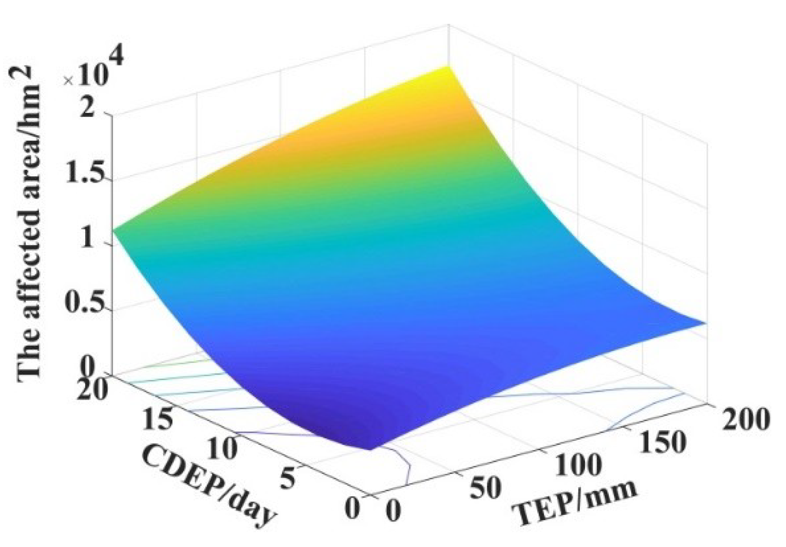
Based on the flood disaster loss data and flood indicators, the flood disaster vulnerability surface model of the MJP was created using the Equations (7)–(9) (Table 5). Its R2 at the 0.05 significance level is 0.6778, which indicates that the model on behalf of the vulnerability of the region is effective and quantitatively signifies the level of agricultural flood vulnerability in the MJP. Figure 6 shows that the extent of the flood damage in the agricultural area increases with TEP and CDEP. The main reason for this was found in the statistical data. The CDEP increase is mainly due to the continuous non-cumulative number of days due to extreme precipitation when TEP and CDEP increase, while the intensity of extreme precipitation in a single events trend to huge. However, the intensity of the extreme events poses greater risks for crops than that of non-extreme precipitation events. The greater the intensity of the extreme precipitation and quantity of ground water are, the greater is the probability of flooding. The weather was not conducive to sustained rainfall and the growth of crops, and could easily lead to crop reduction.
3.4. Risk Curves
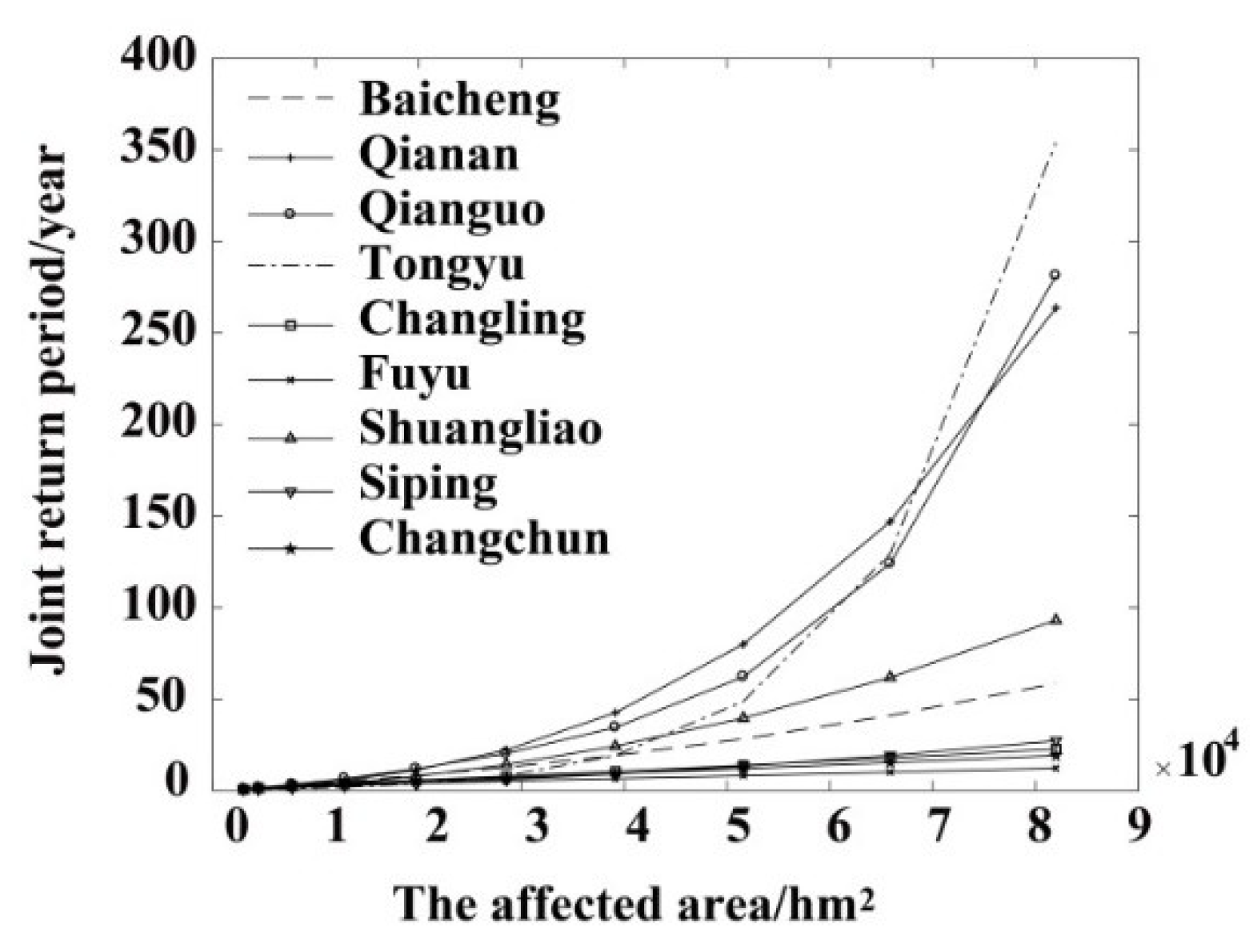
The agricultural flood disaster risk curve of the MJP was determined in this study based on the joint distribution and vulnerability surface model (Figure 7). As seen in the figure, the horizontal axis represents the flood-affected area of agriculture and the vertical axis indicates the joint return period. At the same situation of the affected area, the lower the joint return period, the greater the flood risk in the study area. We can infer from the risk curve that the agricultural flood risk of the MJP generally presented a rule of high in the east and low in the west. The high-risk areas include Fuyu, followed by Changchun, Changling, Siping, Baicheng, and Shuangliao. As the affected area increased, the curve of these areas does not increase much, indicating that the joint return period of the CDEP and TEP is lower and prone to flooding. In contrast, the flood risk in Qianan, Qianguo, and Tongyu is relatively low. The curves increase significantly as the flood-affected area increases, which indicate that the two indices have a lower joint return period and are less prone to flooding. The results can provide a scientific basis for flood control and drainage plans in the area.
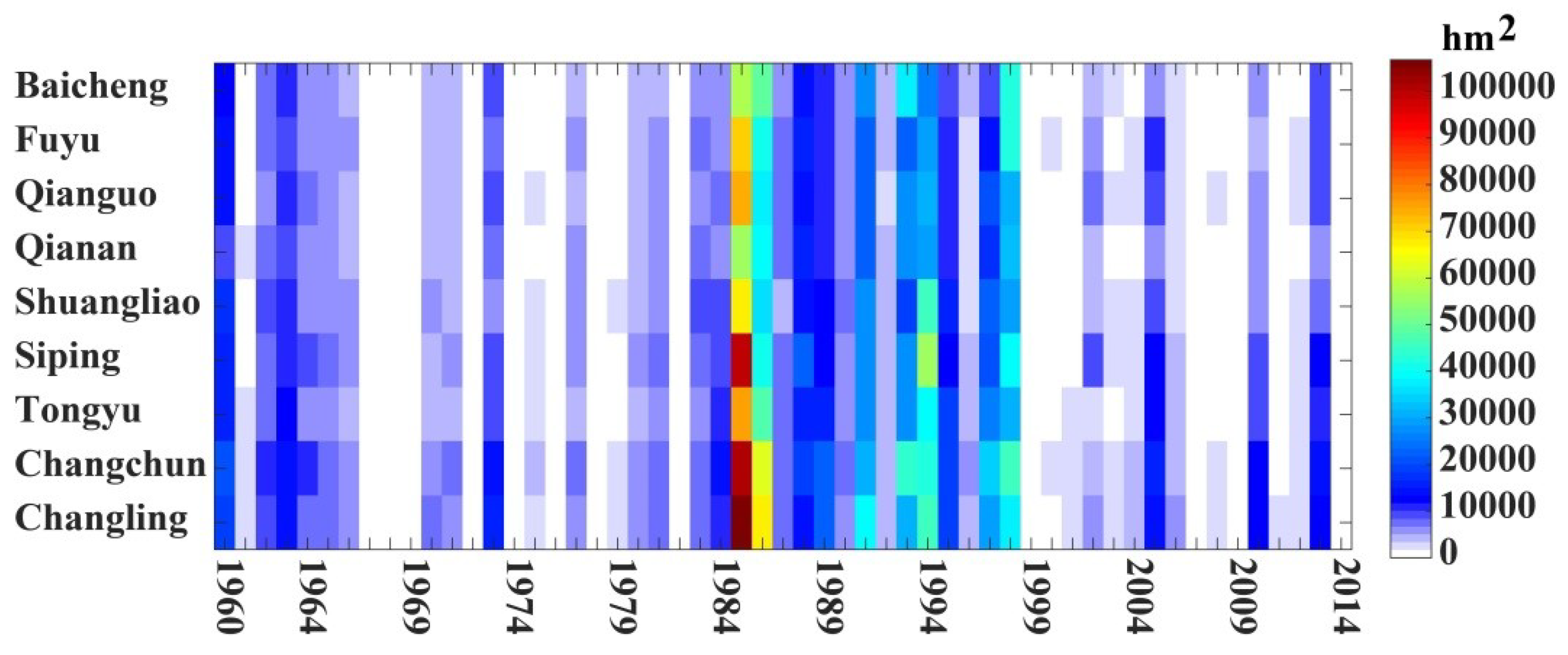
The historical flood-affected area of nine counties in the MJP from 1960 to 2014 was analysed in this study to verify the accuracy of the risk curve model (Figure 8). Flood disasters seriously impacted the area (Figure 8). The return period of flood is approximately six years (calculated by the risk curve model) when the affected area is 1 × 10⁴ hm2. The comparison of the simulated values and historical statistics indicates seven or eight flood disasters for each county. In other words, flood disasters occurred every seven to eight years between 1960 and 2014 in the MJP. Although the simulated values were smaller than the observed data, this implies that the proposed model for the flood risk assessment is highly accurate and efficient.
4. Discussion
Using the data of the joint return period of CDEP and TEP and the flood affected area of nine administrative units in the study area, the flood risk curves for crops in the MJP were constructed. We found that high-levels of agricultural flood risk is mainly concentrated in the eastern region of the study area, including Changchun and Fuyu. Sun has built a risk assessment index system for storms and floods in the Jilin Province from the four aspects of hazard of the disaster-causing factors, sensitivity of the disaster-breeding environment, vulnerability of the hazard affected body, and disaster prevention and mitigation capabilities. They have also found Changchun is a high-risk area of heavy storms and floods [47]. Although some differences were noted in the data and methods, the results of our study are generally consistent with that of Sun. Globally, a large increase in flood frequency in Southeast Asia, Peninsular India, eastern Africa, and the northern half of the Andes was demonstrated by Hirabayashi et al. They also revealed that the global exposure to floods would increase depending on the degree of warming [48]. For Asia, Jung et al. constructed the flood risk index (FRI), considering the natural factors, social factors, administrative and economic factors, and facility factors. They found that the FRI was high in the southeastern coastal region and basins of the two biggest rivers in South Korea [49]. Shaikh et al. believed that the education level and environmental awareness of the coastal area people has a close relationship with the activities during flood disaster in flood disaster risk reduction and adaptation in Bangladesh [50]. For China, Xu et al. have found that high flood risks will mainly appear in the in major part of East China, the major cities in Northeast China, as well as the coastal areas in southeastern China under the Representative Concentration Pathway (RCP) 8.5 scenario [51]. Similar to the method used in our article, Ming et al. assessed the risk of crop losses in the Yangtze River Delta region, China using the vulnerability surface and joint return period of hazards. They selected the joint return period of wind speed and rainfall as intensity of the hazards and built a vulnerability surface of crops in multi-hazards [30]. In our study, we established a vulnerability surface of crops with data of the CDEP, TEP, and flood affected area. The advantage of this model is that it can express the flood loss under multi-hazard factors, and can derive the intensity (joint return period) of multi-hazards in the same flood loss scenarios. The ability to estimate the expected loss of crops in a multi-hazard scenario is of great value in risk management, including agricultural planning and agricultural insurance.
Floods are inevitable and recurring natural disasters associated with extreme precipitation events and the looming climate change [48]. Climate change, characterized by global warming, is now thought to exacerbate the hydrological cycle, change the temporal and spatial patterns of precipitation, and increase the occurrence of extreme precipitation, such as floods and droughts [52]. Agriculture is the second largest source of carbon emissions in modern society [53]. Therefore, using some low-carbon agricultural technologies [54] to reduce carbon emissions is an effective way to adapt to the future climate warming and effectively prevent extreme precipitation events, including floods. According to the research results of this paper and the characteristics of the agricultural environment of the study area, we believe that some engineering measures should be taken in areas with high flood risk. For example, the combination of conservation tillage and straw returning technology can reduce soil weathering strength, regulate soil temperature, and enhance soil moisture retention. The use of compound fertilizers and organic fertilizers can balance soil nutrients, increase soil fertility and yield, and reduce carbon emissions. Reasonable use of cover film insulation and water temperature regulation technology can reduce the probability of water loss in the field. On the other hand, non-engineering measures for flood prevention and mitigation should be strengthened for areas with low flood risk. For example, the education and publicity work on the prevention and control of agricultural meteorological disasters can enable residents to raise awareness of agricultural flood prevention. Constructing and improving an efficient and reliable flood control command system can effectively predict and monitor flood information. The implementation of these measures cannot be separated from the support and supervision of government departments. They should regularly check and promptly identify problems and countermeasures to achieve the purpose of disaster prevention and mitigation.
It should be noted that the main weakness of this study is the failure to address the quantitative relationship between the intensity and duration of extreme precipitation events and the flood, including underlying surface factors affecting agricultural floods. Although the conclusions drawn in this paper are consistent with the actual situation over time, it is necessary to explore the mechanism of flood disaster caused by extreme precipitation so as to select the most appropriate indicators for risk assessment of agricultural flood disaster. In addition, the lack of sample data when constructing vulnerability surfaces is also one of the limitations of the paper. Generally, the more sample data of the input model, the more inaccurate the research results. However, the problem of missing data often occurs in existing historical records. Therefore, we can adjust the model parameters in future research work and use other types of data to conduct agricultural flood risk research. In terms of flood hazard factors, we can use the remote sensing inversion method to extract the flood depth and duration, and build a vulnerability surface of flood hazard factors for underlying surface factors and disaster loss data. In terms of disaster loss data, we can use field trials to observe crop growth in a set scenario or use some crop models to simulate the crop loss under the different flood intensity and duration. Furthermore, the vulnerability surface model can also can be adapted and applied in other agricultural meteorological disaster risk assessments, such as the agricultural drought risk under multi-hazards.
5. Conclusions
In this study, the total extreme precipitation (TEP) and the number of consecutive days with precipitation ≥0.1 mm during extreme precipitation events (CDEP) were chosen as flood indicators based on the characteristics of the flood events in the MJP. The MF-DFA method used was introduced to define the threshold of extreme precipitation events while the copula function was applied to evaluate the joint probability distribution of the CDEP and TEP, which were used to describe the flood hazards, respectively. Then, the vulnerability surface model was presented using the historical flood data and the joint return period to assess the flood vulnerability of the MJP. Finally, flood risk curves were generated from the aforementioned methods. The main conclusions are as below:
- (1)
- The CDEP and TEP both had a tendency of increase in the MJP. The threshold of extreme precipitation events gradually decreases from east to west, and their spatial distribution is similar to that of the precipitation in this region. The CDEP highly correlates with the TEP at each station and all correlation coefficients pass the 0.05 significance test;
- (2)
- The shortest joint return period was determined for Fuyu and Changchun, which indicates that the flood hazard level of the two regions is higher. On contrary, the longest joint return period was obtained for Tongyu and Qianguo at the same intensity of flood indicators; and
- (3)
- We found that the agricultural flood risk of the MJP gradually decreases from east to west, and the spatial distribution of risk in the area with the same spatial pattern of that of the flood hazard, which further illustrates that the amount and duration of extreme precipitation are the important factors affecting agricultural losses in the region.
Author Contributions
G.L. was responsible for the original idea and the theoretical aspects of the paper. E.G. was responsible for the software while X.Y. was responsible for the data curation. Y.W. drafted the manuscript and all authors read and revised the manuscript.
Funding
This study was supported by the Science and Technology Innovation Project “Grassland Non-biological Disaster Prevention and Mitigation Team” of Chinese Academy of Agricultural Sciences (Grant No. CAAS-ASTIP-IGR2015-04); National Science Foundation for Young Scientists of China (Grant No. 41807507); China the Science and Technology Project of Inner Mongolia Autonomous Region (Grant No. 201502095); Postdoctoral Science Foundation Funded Project (Grant No. 2017M620975).
Conflicts of Interest
The authors declare no conflict of interest.
References
- Mishra, A.K.; Singh, V.P. A Review of Drought Concepts. J. Hydrol. 2010, 391, 202–216. [Google Scholar] [CrossRef]
- Change, C. Mitigation of Climate Change; Contribution of Working Group III to the Fifth Assessment Report of the Intergovernmental Panel on Climate Change; Cambridge University Press: Cambridge, UK; New York, NY, USA, 2014. [Google Scholar]
- Wang, Y.; Zhang, Q.; Singh, V.P. Spatiotemporal Patterns of Precipitation Regimes in the Huai River Basin, China, and Possible Relations with ENSO Events. Nat. Hazards 2016, 82, 2167–2185. [Google Scholar] [CrossRef]
- Zhang, Q.; Wang, Y.; Singh, V.P.; Gu, X.; Kong, D.; Xiao, M. Impacts of ENSO and ENSO Modoki+A Regimes on Seasonal Precipitation Variations and Possible Underlying Causes in the Huai River Basin, China. J. Hydrol. 2016, 533, 308–319. [Google Scholar] [CrossRef]
- Wang, Z.; Lai, C.; Chen, X.; Yang, B.; Zhao, S.; Bai, X. Flood Hazard Risk Assessment Model Based on Random Forest. J. Hydrol. 2015, 527, 1130–1141. [Google Scholar] [CrossRef]
- Jonkman, S.N.; Kok, M.; Vrijling, J.K. Flood Risk Assessment in the Netherlands: A Case Study for Dike Ring South Holland. Risk Anal. 2008, 28, 1357–1374. [Google Scholar] [CrossRef] [PubMed]
- Tapia-Silva, F.O.; Itzerott, S.; Foerster, S.; Kuhlmann, B.; Kreibich, H. Estimation of Flood Losses to Agricultural Crops Using Remote Sensing. Phys. Chem. Earth 2011, 36, 253–265. [Google Scholar] [CrossRef]
- Domeneghetti, A.; Carisi, F.; Castellarin, A.; Brath, A. Evolution of Flood Risk over Large Areas: Quantitative Assessment for the Po River. J. Hydrol. 2015, 527, 809–823. [Google Scholar] [CrossRef]
- Ma, L. Design and Implementation of Multi-Scale Flood Disaster Risk Assessment Model Based on GIS; Capital Normal University: Beijing, China, 2011. (In Chinese) [Google Scholar]
- Yan, S. National Flood Disaster in 2013. China Flood Drought Manag. 2014, 20, 18–19. (In Chinese) [Google Scholar]
- National Flood Control and Drought Relief Headquarters. China Water and Drought Disaster Bulletin in 2013; China Water Conservancy and Hydropower Press: Beijing, China, 2014. (In Chinese) [Google Scholar]
- Gao, F.; Dong, L.; Zhang, B. Characteristics Analysis of Flood Disasters in Jilin Province in the 1990s. Meteorol. Disaster Prev. 2002, 10, 14–17. (In Chinese) [Google Scholar]
- Li, J.; Ren, H.; Liu, S.; Tang, X. Quantitative Analysis of Remote Sensing Monitoring Information of Heavy Rain and Flood Disasters in Jilin Province in Summer of 2010. Meteorol. Disaster Prev. 2012, 19, 38–41. (In Chinese) [Google Scholar]
- Förster, S.; Kuhlmann, B.; Lindenschmidt, K.E.; Bronstert, A. Assessing Flood Risk for a Rural Detention Area. Nat. Hazard. Earth Syst. 2008, 8, 311–322. [Google Scholar] [CrossRef]
- Lei, X.; Zhang, Q.; Zhou, A.L.; Ran, H. Assessment of Flood Catastrophe Risk for Grain Production at the Provincial Scale in China Based on the BMM Method. J. Integr. Agric. 2013, 12, 2310–2320. [Google Scholar]
- Sun, Z.; Liu, X.; Zhu, X.; Pan, Y. Agriculture Flood Risk Assessment Based on Information Diffusion. In Proceedings of the IEEE Geoscience and Remote Sensing Symposium (IGARSS), Beijing, China, 10–15 July 2016; pp. 4391–4394. [Google Scholar]
- Gain, A.K.; Mojtahed, V.; Biscaro, C.; Balbi, S.; Giupponi, C. An Integrated Approach of Flood Risk Assessment in the Eastern Part of Dhaka city. Nat. Hazards 2015, 79, 1499–1530. [Google Scholar] [CrossRef]
- Duan, H.L.; Wang, C.L.; Tang, L.S.; Chen, H. Risk Assessments of Late Rice Flood Disaster in South China. Chin. J. Ecol. 2014, 33, 1368–1373. (In Chinese) [Google Scholar]
- Ghosh, A.; Kar, S.K. Application of Analytical Hierarchy Process (AHP) for Flood Risk Assessment: A Case Study in Malda District of West Bengal, India. Nat. Hazards 2018, 1–20. [Google Scholar] [CrossRef]
- Guo, E.; Zhang, J.; Ren, X.; Zhang, Q.; Sun, Z. Integrated Risk Assessment of Flood Disaster Based on Improved Set Pair Analysis and the Variable Fuzzy Set Theory in Central Liaoning Province, China. Nat. Hazards 2014, 74, 947–965. [Google Scholar] [CrossRef]
- Derdous, O.; Djemili, L.; Bouchehed, H.; Tachi, S.E. A GIS Based Approach for the Prediction of the Dam Break Flood Hazard—A Case Study of Zardezas Reservoir “Skikda, Algeria”. J. Water Land Dev. 2015, 7, 15–20. [Google Scholar] [CrossRef]
- Luu, C.; Meding, J.V.; Kanjanabootra, S. Assessing Flood Hazard Using Flood Marks and Analytic Hierarchy Process Approach: A Case Study for the 2013 Flood Event in Quang Nam, Vietnam. Nat. Hazards 2018, 90, 1031–1050. [Google Scholar] [CrossRef]
- Wu, F.; Sun, Y.; Sun, Z.; Wu, S.; Zhang, Q. Assessing Agricultural System Vulnerability to Floods: A Hybrid Approach Using Emergy and a Landscape Fragmentation Index. Ecol. Indic. 2017. [Google Scholar] [CrossRef]
- Paprotny, D.; Sebastian, A.; Morales-Nápoles, O.; Jonkman, S.N. Trends in Flood Losses in Europe over the Past 150 Years. Nat. Commun. 2018, 9, 1985. [Google Scholar] [CrossRef] [PubMed]
- Salman, A.M.; Li, Y. Flood Risk Assessment, Future Trend Modeling, and Risk Communication: A Review of Ongoing Research. Nat. Hazards Rev. 2018, 19, 04018011. [Google Scholar] [CrossRef]
- Hsu, W.K.; Huang, P.C.; Chang, C.C.; Chen, C.W.; Hung, D.M.; Chiang, W.L. An Integrated Flood Risk Assessment Model for Property Insurance Industry in Taiwan. Nat. Hazards 2011, 58, 1295–1309. [Google Scholar] [CrossRef]
- Papathoma-Koehle, M.; Keiler, M.; Totschnig, R.; Glade, T. Improvement of Vulnerability Curves Using Data from Extreme Events: Debris Flow Event in South Tyrol. Nat. Hazards 2012, 64, 2083–2105. [Google Scholar] [CrossRef]
- Zischg, A.P.; Felder, G.; Weingartner, R.; Quinn, N.; Coxon, G.; Neal, J.; Freer, J.; Bates, P. Effects of Variability in Probable Maximum Precipitation Patterns on Flood Losses. Hydrol. Earth Syst. Sci. 2018, 22, 2759–2773. [Google Scholar] [CrossRef]
- Madsen, H.; Lawrence, D.; Lang, M.; Martinkova, M.; Kjeldsen, T.R. Review of Trend Analysis and Climate Change Projections of Extreme Precipitation and Floods in Europe. J. Hydrol. 2014, 519, 3634–3650. [Google Scholar] [CrossRef] [Green Version]
- Ming, X.; Xu, W.; Li, Y.; Du, J.; Liu, B.; Shi, P. Quantitative Multi-Hazard Risk Assessment with Vulnerability Surface and Hazard Joint Return Period. Stoch. Environ. Res. Risk Assess. 2015, 29, 35–44. [Google Scholar] [CrossRef]
- Zhao, J.; Guo, J.; Xu, Y.; Mu, J. Effects of Climate Change on Cultivation Patterns of Spring Maize and Its Climatic Suitability in Northeast China. Agric. Ecosyst. Environ. 2015, 202, 178–187. [Google Scholar] [CrossRef]
- Guo, E.; Zhang, J.; Wang, Y.; Alu, S.; Wang, R.; Li, D.; Ha, S. Assessing Non-Linear Variation of Temperature and Precipitation for Different Growth Periods of Maize and their Impacts on Phenology in the Midwest of Jilin Province, China. Theor. Appl. Climatol. 2018, 132, 685–699. [Google Scholar] [CrossRef]
- Wen, K. Chinese Meteorological Disasters Ceremony (Jilin Volume); China Meteorological Press: Beijing, China, 2008. (In Chinese) [Google Scholar]
- Kantelhardt, J.W.; Zschiegner, S.A.; Koscielny-Bunde, E.; Havlin, S.; Bunde, A.; Stanley, H.E. Multifractal Detrended Fluctuation Analysis of Nonstationary Time Series. Physica A 2002, 316, 87–114. [Google Scholar] [CrossRef]
- Du, H.; Wu, Z.; Zong, S.; Meng, X.; Wang, L. Assessing the Characteristics of Extreme Precipitation over Northeast China Using the Multifractal Detrended Fluctuation Analysis. J. Geophys. Res. 2013, 118, 6165–6174. [Google Scholar] [CrossRef]
- Du, H.; Wu, Z.; Li, M.; Jin, Y.; Zong, S.; Meng, X. Characteristics of Extreme Daily Minimum and Maximum Temperature over Northeast China, 1961–2009. Theor. Appl. Climatol. 2013, 111, 161–171. [Google Scholar] [CrossRef]
- Baranowski, P.; Krzyszczak, J.; Slawinski, C.; Hoffmann, H.; Kozyra, J.; Nieróbca, A.; Gluza, A. Multifractal Analysis of Meteorological Time Series to Assess Climate Impacts. Clim. Res. 2015, 65, 39–52. [Google Scholar] [CrossRef]
- Guo, E.; Zhang, J.; Si, H.; Dong, Z.; Cao, T.; Lan, W. Temporal and Spatial Characteristics of Extreme Precipitation Events in the Midwest of Jilin Province Based on Multifractal Detrended Fluctuation Analysis Method and Copula Functions. Theor. Appl. Climatol. 2016, 130, 597–607. [Google Scholar] [CrossRef]
- Timonina, A.; Hochrainer-Stigler, S.; Pflug, G.; Jongman, B.; Rojas, R. Structured Coupling of Probability Loss Distributions: Assessing Joint Flood Risk in Multiple River Basins. Risk Anal. 2015, 35, 2102–2119. [Google Scholar] [CrossRef] [PubMed]
- Li, N.; Liu, X.; Xie, W.; Wu, J.; Zhang, P. The Return Period Analysis of Natural Disasters with Statistical Modeling of Bivariate Joint Probability Distribution. Risk Anal. 2013, 33, 134–145. [Google Scholar] [CrossRef] [PubMed]
- Wang, C.; Ren, X.; Li, Y. Analysis of Extreme Precipitation Characteristics in Low Mountain Areas Based on Three-dimensional Copulas—Taking Kuandian County as an Example. Theor. Appl. Climatol. 2015, 128, 169–179. [Google Scholar] [CrossRef]
- Murray, A.T. Quantitative geography. J. Reg. Sci. 2010, 50, 143–163. [Google Scholar] [CrossRef]
- Bernaola-Galván, P.; Ivanov, P.C.; Amaral, L.A.N.; Stanley, H.E. Scale Invariance in the Nonstationarity of Human Heart Rate. Phys. Rev. Lett. 2001, 87, 168105. [Google Scholar] [CrossRef] [PubMed]
- Ren, B.; Zhang, J.; Li, X.; Fan, X.; Dong, S.; Liu, P.; Zhao, B. Effects of Waterlogging on the Yield and Growth of Summer Maize under Field Conditions. Can. J. Plant. Sci. 2014, 94, 23–31. [Google Scholar] [CrossRef]
- International Strategy for Disaster Reduction. Living with Risk: A Global Review of Disaster Reduction Initiatives; United Nations Press: New York, NY, USA, 2004. [Google Scholar]
- Liu, X.; Zhang, J.; Ma, D.; Bao, Y.; Tong, Z.; Liu, X. Dynamic Risk Assessment of Drought Disaster for Maize Based on Integrating Multi-sources Data in the Region of the Northwest of Liaoning Province, China. Nat. Hazards 2013, 65, 1393–1409. [Google Scholar] [CrossRef]
- Sun, J. Risk Assessment of Rainstorm and Flood Disaster in Jilin Province Based on GIS and RS Technology; Northeast Normal University: Changchun, China, 2010. (In Chinese) [Google Scholar]
- Hirabayashi, Y.; Mahendran, R.; Koirala, S.; Konoshima, L.; Dai, Y.; Watanabe, S.; Kim, H.; Kanae, S. Global flood risk under climate change. Nat. Clim. Chang. 2013, 3, 816–821. [Google Scholar] [CrossRef]
- Jung, Y.; Shin, Y.; Jang, C.H.; Kum, D.; Kim, Y.S.; Lim, K.J.; Kim, H.B.; Park, T.S.; Lee, S.O. Estimation of Flood Risk Index Considering the Regional Flood Characteristics: A Case of South Korea. Paddy Water Environ. 2014, 12, 41–49. [Google Scholar] [CrossRef]
- Shaikh, M.S.; Shariot-Ullah, M.; Ali, M.A.; Adham, A.K.M. Flood Disaster Risk Reduction and Adaptation around the Coastal Area of Bangladesh. J. Environ. Sci. Nat. Resour. 2015, 6, 53–57. [Google Scholar] [CrossRef]
- Ying, X.U.; Zhang, B.; Zhou, B.T.; Dong, S.Y.; Li, Y.U.; Rou-Ke, L.I. Projected Flood Risks in China Based on Cmip5. Adv. Clim. Chang. Res. 2014, 5, 57–65. [Google Scholar] [CrossRef]
- Vörösmarty, C.J.; McIntyre, P.B.; Gessner, M.O.; Dudgeon, D.; Prusevich, A.; Green, P.; Davies, P.M. Global Threats to Human Water Security and River Biodiversity. Nature 2010, 467, 555–561. [Google Scholar] [CrossRef] [PubMed]
- Zhang, X.; Han, S.; Xu, Q. The Application Intention and Driving Factors of Agricultural Low-Carbon Technology: Based on the Investigation of Scale Farmers in Jiangxi. Chin. J. Ecol. Econ. 2018, 34, 54–60. (In Chinese) [Google Scholar]
- Norse, D. Low Carbon Agriculture: Objectives and Policy Pathways. Environ. Dev. 2012, 1, 25–39. [Google Scholar] [CrossRef]
Figure 1.
Location map of the study area in China.

Figure 2.
Temporal variations of the main types of crops in the MJP. (a) variation characteristics of maize yield; (b) variation characteristics of rice yield; (c) variation characteristics of soybean yield; (d) the proportions of individual crops area.
Figure 2.
Temporal variations of the main types of crops in the MJP. (a) variation characteristics of maize yield; (b) variation characteristics of rice yield; (c) variation characteristics of soybean yield; (d) the proportions of individual crops area.

Figure 3.
Schematic diagram of flood indicators.

Figure 4.
Comparison of the observed samples and the fitted marginal distributions of CDEP and TEP.

Figure 5.
The joint return period of CDEP and TEP.

Figure 6.
Vulnerability surface of crops in the MJP.

Figure 7.
Flood risk curves for crops in the MJP.

Figure 8.
The historical flood-effected area of nine counties in the MJP from 1960 to 2014.


Table 1.
Bivariate Archimedean copula function and parameter space.
| Copula Function | Parameter Space | |
|---|---|---|
| Frank Copula | ||
| Clayton Copula | ||
| Gumbel Copula |
Table 2.
The threshold of extreme precipitation events.
| Stations | Changchun | Tongyu | Changling | Qianan | Qianguo | Shuangliao | Fuyu | Baicheng | Siping |
|---|---|---|---|---|---|---|---|---|---|
| threshold | 47.8 | 38.3 | 48.2 | 38.4 | 37.1 | 58.5 | 43 | 38.5 | 56.6 |
Table 3.
The fitting parameters for the marginal distribution of the flood indicators.
| Indicators | Parameters | Changchun | Tongyu | Changling | Qianan | Qianguo | Shuangliao | Fuyu | Baicheng | Siping |
|---|---|---|---|---|---|---|---|---|---|---|
| TEP | k | 0.375 | 0.200 | 0.295 | −0.026 | 0.844 | 0.808 | 0.337 | 0.498 | 0.674 |
| s | 45.635 | 45.170 | 39.520 | 44.960 | 29.917 | 44.423 | 37.930 | 47.953 | 45.413 | |
| m | 84.566 | 91.208 | 79.495 | 94.979 | 71.990 | 81.112 | 94.069 | 100.317 | 96.017 | |
| CDEP | k | 0.302 | 0.250 | −0.183 | 0.171 | 0.469 | 0.527 | 0.606 | 0.319 | 0.539 |
| s | 2.464 | 2.149 | 2.485 | 2.039 | 1.709 | 2.241 | 1.577 | 1.967 | 2.248 | |
| m | 3.433 | 3.545 | 3.946 | 3.187 | 2.425 | 3.407 | 2.387 | 3.363 | 3.302 |
Table 4.
Selection of the copula function and parameters.
| Stations | Copula Functions | RMSE | AIC | Parameter |
|---|---|---|---|---|
| Baicheng | Clayton | 0.0653 | −116.9052 | 1.4973 |
| Frank | 0.0533 | −125.8407 | 7.1460 | |
| Gumbel | 0.0501 | −128.6466 | 2.4672 | |
| Qianan | Clayton | 0.0679 | −115.1339 | 0.9138 |
| Frank | 0.0529 | −126.1794 | 4.8031 | |
| Gumbel | 0.0500 | −128.6915 | 1.8931 | |
| Qianguo | Clayton | 0.0541 | −125.2456 | 2.0720 |
| Frank | 0.0530 | −126.1135 | 7.4039 | |
| Gumbel | 0.0521 | −126.8485 | 2.5475 | |
| Tongyu | Clayton | 0.0617 | −119.3877 | 1.8507 |
| Frank | 0.0627 | −118.6967 | 6.7939 | |
| Gumbel | 0.0712 | −113.0363 | 2.0599 | |
| Changling | Clayton | 0.0603 | −120.4239 | 1.8507 |
| Frank | 0.0520 | −126.9380 | 6.7939 | |
| Gumbel | 0.0511 | −127.7760 | 2.0599 | |
| Fuyu | Clayton | 0.0547 | −124.7080 | 2.2624 |
| Frank | 0.0510 | −127.7962 | 9.1288 | |
| Gumbel | 0.0506 | −128.1797 | 2.8739 | |
| Shuangliao | Clayton | 0.0652 | −116.9382 | 0.9143 |
| Frank | 0.0566 | −123.1843 | 4.4784 | |
| Gumbel | 0.0540 | −125.2837 | 1.8775 | |
| Siping | Clayton | 0.0615 | −119.5317 | 1.5214 |
| Frank | 0.0578 | −122.2900 | 6.6635 | |
| Gumbel | 0.0542 | −125.0960 | 2.4773 | |
| Changchun | Clayton | 0.0738 | −111.4586 | 1.3408 |
| Frank | 0.0568 | −123.0482 | 7.4784 | |
| Gumbel | 0.0551 | −124.3642 | 2.6622 |
Note: Italic font indicates the selected copula function based on values of the AIC and RMSE.
Table 5.
Estimated values of coefficients in the vulnerability model.
| Coefficient | a | b | C | d | e | f |
|---|---|---|---|---|---|---|
| Estimated Value | 3421 | −32.14 | 292.9 | 0.3552 | 0.7325 | −7.738 |
© 2018 by the authors. Licensee MDPI, Basel, Switzerland. This article is an open access article distributed under the terms and conditions of the Creative Commons Attribution (CC BY) license (http://creativecommons.org/licenses/by/4.0/).
Share and Cite
MDPI and ACS Style
Wang, Y.; Liu, G.; Guo, E.; Yun, X. Quantitative Agricultural Flood Risk Assessment Using Vulnerability Surface and Copula Functions. Water 2018, 10, 1229. https://doi.org/10.3390/w10091229
AMA Style
Wang Y, Liu G, Guo E, Yun X. Quantitative Agricultural Flood Risk Assessment Using Vulnerability Surface and Copula Functions. Water. 2018; 10(9):1229. https://doi.org/10.3390/w10091229
Chicago/Turabian StyleWang, Yongfang, Guixiang Liu, Enliang Guo, and Xiangjun Yun. 2018. "Quantitative Agricultural Flood Risk Assessment Using Vulnerability Surface and Copula Functions" Water 10, no. 9: 1229. https://doi.org/10.3390/w10091229
Note that from the first issue of 2016, this journal uses article numbers instead of page numbers. See further details here.