Coupling of Ultrasonic and Photometric Techniques for Synchronous Measurements of Unconfined Turbidity Currents


1
Water Engineering, Tonkin & Taylor Ltd., Auckland 1023, New Zealand
2
Department of Civil and Environmental Engineering, University of Auckland, Auckland 1142, New Zealand
*
Author to whom correspondence should be addressed.
†
Formerly Department of Civil and Environmental Engineering, University of Auckland.
Water 2018, 10(9), 1246; https://doi.org/10.3390/w10091246
Submission received: 13 May 2018
/
Revised: 7 September 2018
/
Accepted: 12 September 2018
/
Published: 14 September 2018
(This article belongs to the Special Issue Water Resources and Environmental Fluid Mechanics: From the Glacier to the Lake/Ocean)
Abstract
:By synchronizing data collection, such as photometric and ultrasonic Doppler profiling (UVP) measurement techniques, new insights can be obtained into environmental flows, such as highly dynamic turbidity currents. We introduce a combined experimental setup, which ultimately allows a time reduction in testing programmes, and discuss the measurement advances with the help of four surface conditions we tested for unconfined turbidity currents: (a) a smooth surface; (b) a smooth surface with an obstacle present; (c) a rough surface; and (d) a rough surface with an obstacle present. We show that data from both measurement techniques indicate that a rough surface reduces global current velocities and the magnitude of turbidity current phenomena, including Kelvin-Helmholtz instabilities and lobe-and-cleft formation. However, by coupling the techniques, photometric data give valuable insight into the spatial development of instabilities, such as the grouping of lobe and cleft formations. The presence of an obstacle causes local regions of an increased and decreased velocity, but does not affect the global current velocity. Additionally, the obstacle created three local intensity maxima upstream, dissipating to two maxima downstream, supporting the presence of local eddies. The study shows that the combination of UVP and photometry is an effective way forward for obtaining detailed qualitative and quantitative insights into turbulent flow characteristics and we highlight the potential for future research.
1. Introduction
Sediment-laden gravity currents, commonly referred to as turbidity currents, are found in sedimentary environments such as seas, deep oceans, reservoirs, and lakes, where they are significant contributors to sediment transport [1]. Density differences between the sediment-laden fluid and surrounding ambient fluid cause the current to propagate. Triggering events can cause these currents to mobilize sediment off the subaqueous bed, causing a catastrophically erosive current [2]. Turbidity currents pose potential environmental hazards, such as submarine cable damage and reservoir sedimentation, and are thus important to engineers [3]. Similarly, turbidity currents are important to scientists as they are one of the main agents of geological sea-bed formation and stratigraphy, which in turn host some of the largest oil reservoirs [4]. Complex numerical solutions of turbidity current mechanics are desired to enable the prediction of long-term events of turbidite formation [2]. In order to validate such models, laboratory experiments are needed, focusing on the flow characteristics of small-scale turbidity currents, e.g., [5].
Through laboratory experiments, Altinakar et al. [6] showed that the vertical velocity profile of density-driven currents is similar to a wall jet, with two key regions; a lower wall region where turbulence is dominated by bottom shear and an upper jet region where shear between the current and ambient fluid occurs, causing the entrainment of ambient fluid (Figure 1). The maximum forward velocity of the current is located at the interface of these two regions, where [7] showed that the interface occurred at a height of z/z1 ≈ 0.2, where z1 is the current height. Kneller et al. [7] also showed that the vertical velocity profile could be represented as the sum of a Gaussian and logarithmic function [8], and conducted a review of velocity and turbulence intensity profiles of previous studies, highlighting the trend of two local intensity peaks either side of the velocity maximum. Furthermore, through detailed photometric experiments, Nogueira et al. [9] showed that the height of gravity currents can be represented as z/z0 ≈ 1/3, where z0 is the ambient fluid height. Their adopted photometric method, previously implemented qualitatively by [10], is a novel advancement for the evaluation of current spatial development, density, and front velocity from a side view.
However, photometry alone cannot measure velocities within the current head and body, hence a coupled measurement approach with in-situ instruments is still needed to also provide insight into velocity and turbulence profiles. In addition, incorporating plan-view photometry allows an interrogation of planar development, which is an important aspect to consider for unconfined currents. Ultrasonic Doppler velocity profiling (UVP) and photometry have become popular measurement techniques for the study of saline and sediment-laden gravity currents. To the authors’ knowledge, no studies have sought to combine the techniques simultaneously to streamline experimental testing programs and remove the error associated with test repetition, which is the objective of this study.
Effect of Confinement and Obstacles on Flow
To highlight the advantage of using a coupled UVP and photometric approach, we revisit research that addresses confinement and obstacles relevant for turbidity currents, as we see this as an area for the major uptake of the combined flow measurement instrumentation. Since [11] related turbidity currents to the damage of submarine structures, limited research has been conducted on how turbidity currents interact with obstacles at a fundamental level [12]. Similarly, better understanding the effect of bed roughness on gravity current dynamics is also gaining more attention in the research community [13,14]. Other research has concentrated on developing a better understanding of the effect of seafloor topography on current behavior [15,16].
Previous research conducted on obstacles has focused on determining the relationship between obstacle height and mass flux of the turbidity current that overpasses the obstacle [17,18,19]. Other studies have focused on developing theoretical models of current interaction with obstacles, based on shallow-water theory [12,20,21,22,23]. More recently, high resolution 3-D models have been developed [24]. However, few experimental studies involving obstacles have investigated the velocity and turbulence structure within the current head.
Oshaghi et al. [25] studied the velocity and concentration profiles of confined quasi-steady turbidity currents of various inlet densimetric Froude numbers interacting with an isosceles triangular obstacle of varying heights. An ADV probe was used to measure velocities at different heights around the obstacle and construct velocity and concentration profiles of the current. The study found that the obstacle reduces the local Froude numbers before the obstacle and increases the local Froude numbers after the obstacle. Interestingly, their profiles showed that the currents increased in velocity after the obstacle, which they attributed to current acceleration over the downstream obstacle face.
Eggenhuisen and McCaffrey [8] used UVP techniques to study the interaction of turbidity currents with a single roughness element located at a range of positions in a confined flume. This was conducted to define how the element altered vertical turbulence intensity distributions, and how the distributions evolved downstream. Vertical turbulence profiles of the current over a smooth surface were found to have a similar character to previous studies, in which two local maxima of intensity occurred directly above and below the vertical location of the maximum horizontal velocity. The shape of the obstructed profiles showed a clear dissimilarity to the unobstructed scenario, having a larger, lower maximum turbulence intensity and no upper maximum present.
Oehy et al. [26] conducted a laboratory investigation of the use of obstacles to halt the propagation of turbidity currents in reservoirs, which are a leading cause of reservoir sedimentation. UVP was used to measure velocity profiles before and after a Gaussian-shaped obstacle. In contrast to [25], the study found that the obstacle caused a considerable reduction in current velocity. This contrast may be attributed to the quasi-steady nature of the currents in [25], where forward momentum forces of the current no longer have to compete with the drag forces caused by ambient fluid displacement at the head.
Whilst the ADV methods of [25] were shown to be effective for obtaining profiles of quasi-steady currents, they have limited applicability to lock-exchange currents due to the ADVs single-point measurement system. Lock-exchange generated turbidity currents have discontinuous flow properties; hence velocity measurements must be collected instantaneously to obtain a discrete, representative velocity profile. UVP is therefore gaining popularity as a method for measuring lock-exchange turbidity currents due to its ability to measure multiple velocity profiles [8,26,27,28]. However, it remains under-utilized for experimental studies incorporating obstacles and substrates.
To the authors’ knowledge, no studies have quantified the velocity and turbulence structure of a turbidity current interacting with an obstacle in an unconfined environment. Such studies are needed to better understand what effect confinement has on the velocity structure and to what extent bed roughness plays a role in velocity and turbulence development. In addition, it is important to consider how obstacles and bed roughness affect the lateral movements of the unconfined current. Confined studies on gravity currents are commonly presented as two-dimensional flows [9,29,30], hence their lateral movements are seldom considered. Lateral movements of unconfined currents interacting with obstacles are of interest. Due to the conservation of mass, variations in radial current velocity surrounding the obstacle may relate to changes in lateral movement. Therefore, a two-dimensional flow representation cannot be assumed for unconfined currents [31]. Photometric tracking of density currents from a side view is becoming a popular measurement technique for confined currents due to technology advances and the ability to obtain high quality images from consumer-grade cameras [30,32,33]. For unconfined currents, photometry can provide pseudo three-dimensional insight into planar development of the current front. However, it remains under-employed [33,34,35,36]. Furthermore, it is uncommon for studies incorporating obstacles [37,38]. Hence, a promising laboratory technique to simultaneously investigate the three-dimensional development of unconfined currents and velocity profiles, is a combination of UVP techniques and photometry.
The presented study therefore has two objectives: Firstly, to develop a process for combining UVP and photometric techniques; and secondly, to investigate what effect a rectangular obstacle and bed roughness have on the velocity and turbulence profiles of an unconfined turbidity current. Ultrasonic techniques are used to evaluate turbidity current flow structure in immediate regions surrounding a rectangular obstacle. Simultaneously, a qualitative photometric technique is applied to visually evaluate lateral current development and provide comparisons with velocity readings. Four different obstacle scenarios are tested: (a) smooth bed without obstacle (NS); (b) smooth bed with obstacle (OS); (c) rough bed without obstacle (NR); and (d) rough bed with obstacle (OR).
2. Experimental Methodology
2.1. Basin and Material
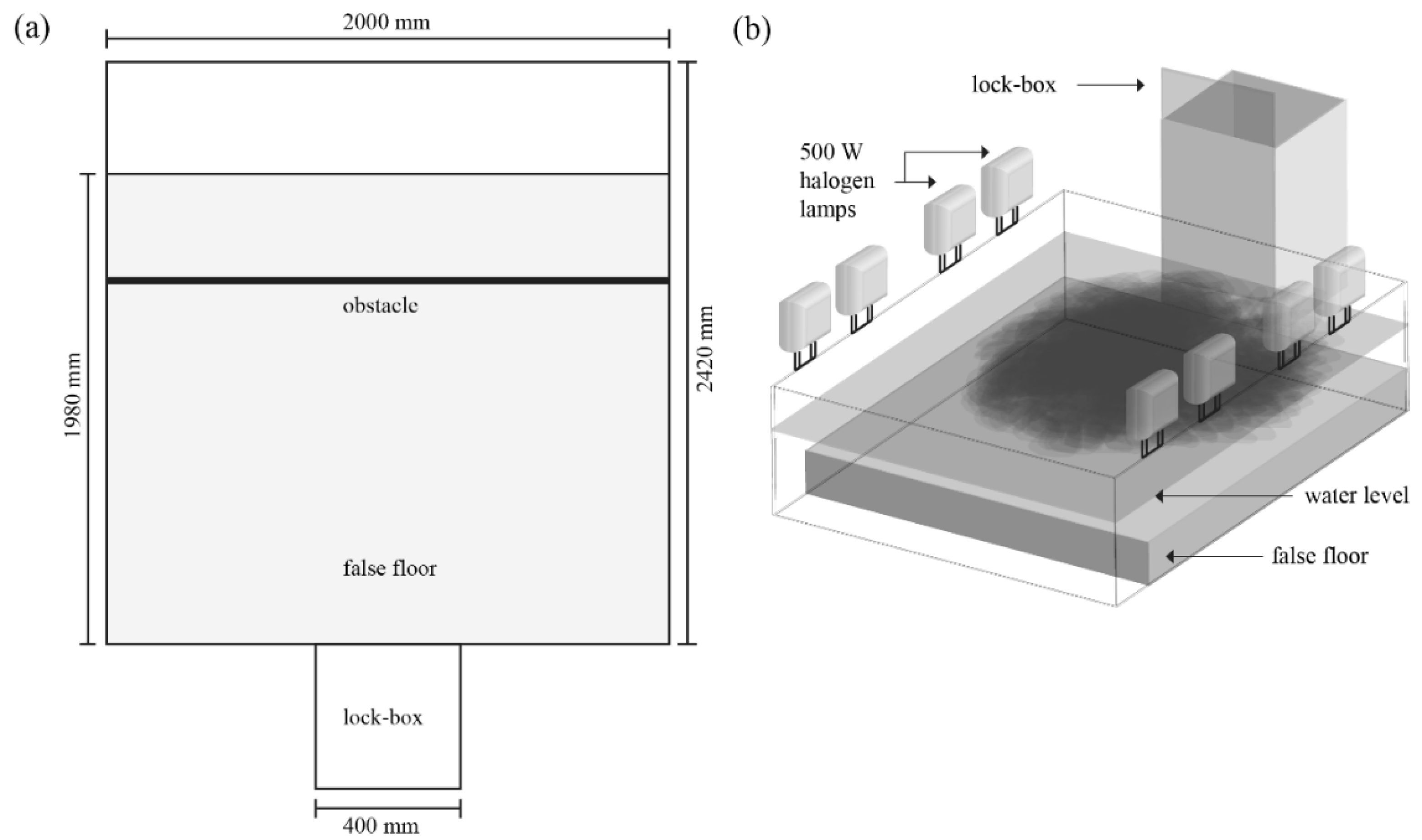
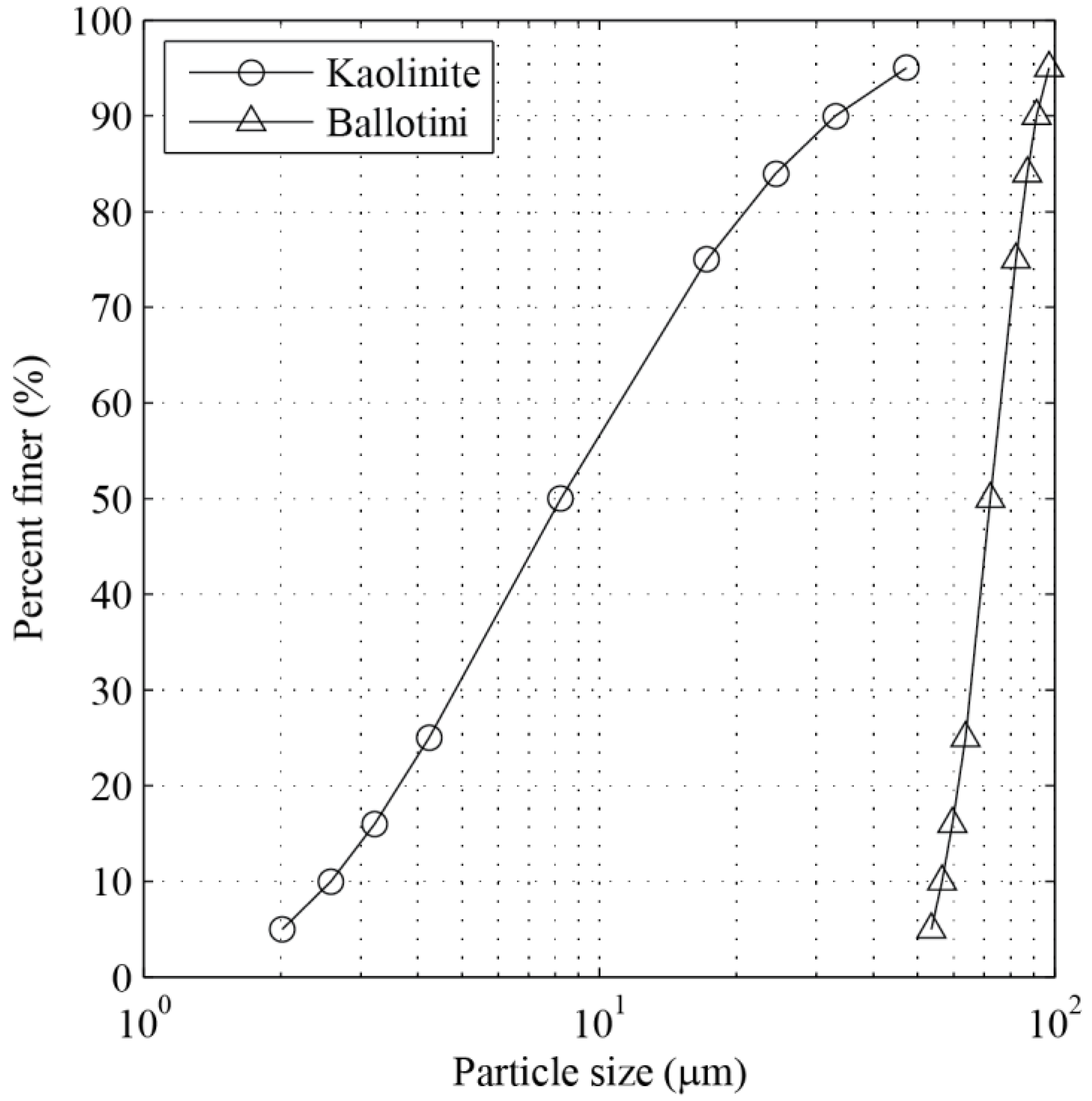
Experimental work was undertaken using a purpose-built 2420 mm long, 2000 mm wide, and 600 mm high (Figure 2) basin in the Water Engineering Laboratory of the University of Auckland. The basin was a hybrid construction of plywood and Perspex, placed on a concrete floor. The use of 12 mm thick Perspex walls along the basin allowed observations from the side. A Perspex lock-box of length x0 = 570 mm, width 400 mm, and height 820 mm was located at the upstream end of the basin. The lock-box had a manual Perspex gate opening into the basin. A false floor made of glass, and positioned 210 mm off the concrete floor, covered a length of 1975 mm from the lock-box. For all tests, the ambient water height, z0, from the false floor was taken as z0 = 265 mm. The turbidity current was composed of a 4% volumetric concentration of kaolinite clay (2%) and Ballotini glass beads (2%), resulting in an initial current density in the range of ρ0 ≈ 1075–1082 kg m−3. A Malvern Mastersizer 2000 was used to determine a grainsize distribution of both sediments (Figure 3).
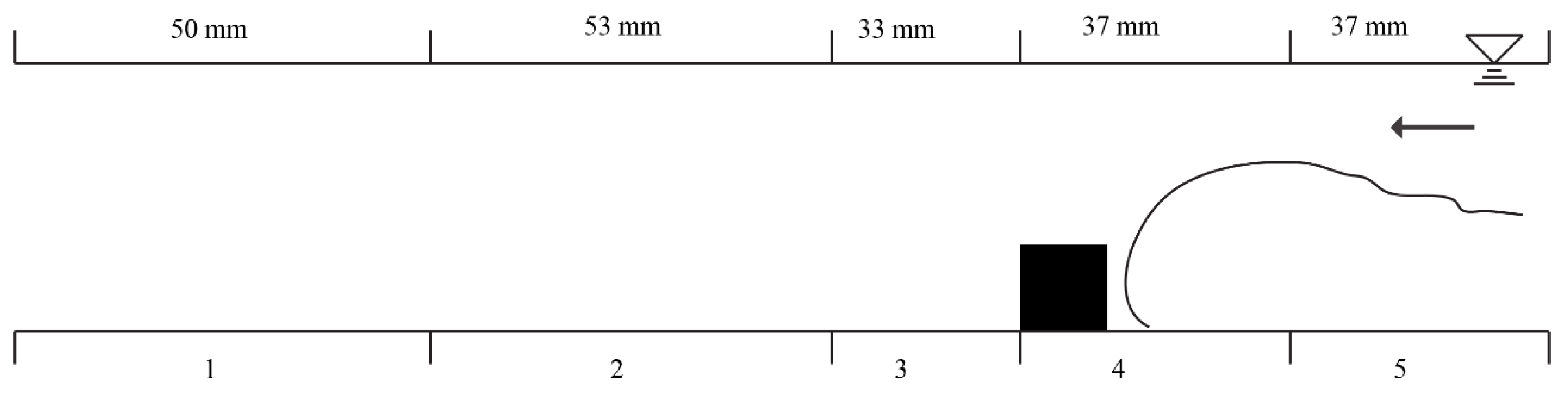
For the four test conditions, the false glass floor acted as the smooth surface. The rough substrate was created using a 4 mm layer of silicon plastic, which had sand of D50 = 0.85 mm glued on the top, and was installed above the glass floor. A 20 mm by 20 mm aluminium square cylinder was used for the two experiments with an obstacle. The rectangular shape was chosen to allow better relation to previous numerical modelling studies, which employ rectangular objects for their simplicity in computations [12]. The obstacle was located along the width of the basin at x/x0 = 2.60 from the lock-box end. This distance was chosen to allow the propagating turbidity current enough time to develop from the slumping phase, but to not invoke a significant interaction with the sidewalls before it reached the obstacle.
2.2. Flow Measurements
A dynamic, qualitative and quantitative analysis of the turbidity current was undertaken by analysing one-dimensional velocity data obtained with a Met-Flow UVP-DUO, set up with 14 transducers. Each 8 mm diameter transducer emits bursts of ultrasonic signals at a frequency of 4 MHz. The signals then travel to a defined number of virtual channels in the fluid, in line with the transducer axis. The signals are reflected off microscopic particles entrained within each virtual channel. The transducer then records the frequency of the reflected signal for each channel, and calculates the change in frequency of the emitted/received signal. Using Doppler theory, the shift in emitted/received frequency is used to calculate the on-axis velocity, u, of the fluid for each channel, creating a velocity profile at each transducer location.
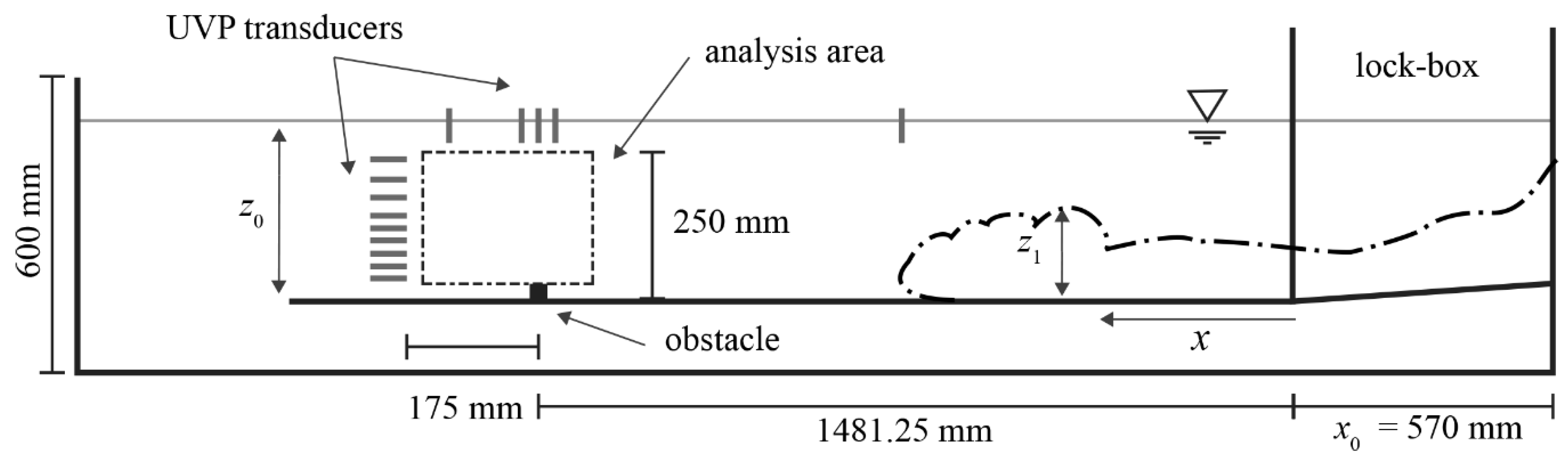
UVP transducers were held horizontally and vertically in a range of positions in the basin by a custom-built Perspex mount, where they had minimal influence on flow. The rig consisted of a vertical section, with machined slots to hold transducers, located near the distal end of the basin, and a horizontal section located 250 mm above the false floor (Figure 4). The sections were located in line with the center of the basin to assure that readings were a symmetrical two-dimensional representation of the current. In past studies, Choux et al. [39] used a vertical array of six horizontal transducers to analyze turbidity currents, whilst [40] used a vertical array of ten transducers. [41], however, used five horizontal and five vertical transducers to obtain two-dimensional velocity vectors within a 25-point grid. For this study, nine horizontally-aligned transducers were stacked in a vertical array facing the approaching current. In addition, five vertical transducers were set up to obtain vertical flow components in five regions. Figure 4 shows the configuration of all 14 transducers. The horizontal (x/x0) and vertical (z/z0) positioning of all transducers are listed in Table 1. Initial tests were conducted to vertically align the transducers with the current head, in a similar setup to [40]. A region of interest in the basin was chosen where all transducers except for transducer #14 were positioned to record horizontal and vertical velocity profiles, as shown in Figure 4. The region of interest was chosen so that the current characteristics immediately before and after the obstacle could be analyzed. Transducer #14 was set up as a reference only and was not used for the analysis. The UVP settings were configured in the initial test runs to ensure that there was a high signal-to-noise ratio (SNR). The settings were similar to those of [41] and adjusted to suit the basin environment (Figure 6). As UVP transducers cannot record simultaneously, they continuously cycle through from transducers #1–14. This caused a trade-off to be present between data quality and time resolution. The number of signal repetitions (number of ultrasonic signals sent per transducer, per profile) can be increased to raise data quality. This, however, results in a longer recording time per transducer. A setting of 32 repetitions was used for the present tests, giving a full cycle time of 1.45 s.
2.3. Photometric Measurements
Static images of the turbidity current were captured using a Nikon D90 camera vertically mounted above the basin from the laboratory ceiling. The camera lens was located 2045 mm from the area of interest. Camera settings were adjusted to maximize shutter speed whilst avoiding the introduction of noise (Table 2). Illumination of the basin was provided by eight 500 W halogen lamps, which were configured to produce an optimum level of contrast in the captured images. Four different lighting scenarios were compared through initial image processing in MATLAB, with the configuration in Figure 2b producing the highest image quality.
2.4. Experimental Procedure
Two test runs were conducted for each obstacle configuration, giving eight individual tests in total. For each run, the basin was filled with tap water to a height of z0 = 265 mm. The slurry was then mechanically mixed whilst the UVP recording process was initiated in synchronization with a stopwatch. At a time of 10 s, a video camera perpendicular to the basin was initiated to record a side view of the turbidity current, and to act as a visual reference. Footage was not used for the analysis. At a time of roughly 18 s, the slurry was poured into the lock-box. The lock-box gate was slowly opened (to reduce disturbance of the ambient water) at a time of 20 s, allowing the turbidity current to freely propagate towards the analysis area. Upon opening of the lock-box, the camera was triggered using a remote switch.
3. Analytical Methodology
3.1. Flow Data
Processing of the UVP data was undertaken in a series of MATLAB programs. The raw velocity data were first filtered for unwanted spikes and noise by adopting a de-spiking method similar to that used by [42]. Velocities obtained from each transducer for all cycles were ordered chronologically for each individual channel. Due to the inconsistent characteristics of the current, a time-wise standard deviation of each channel was applied using an 11-point moving mean. A three-point moving mean replaced all data outlying two standard deviations, which was the same limit used by [42]. This removed most noise spikes without altering more than 6% of data for all four obstacle configurations, which was considered acceptable. An alteration of more than 10% required further optimization of the transducers prior to testing.
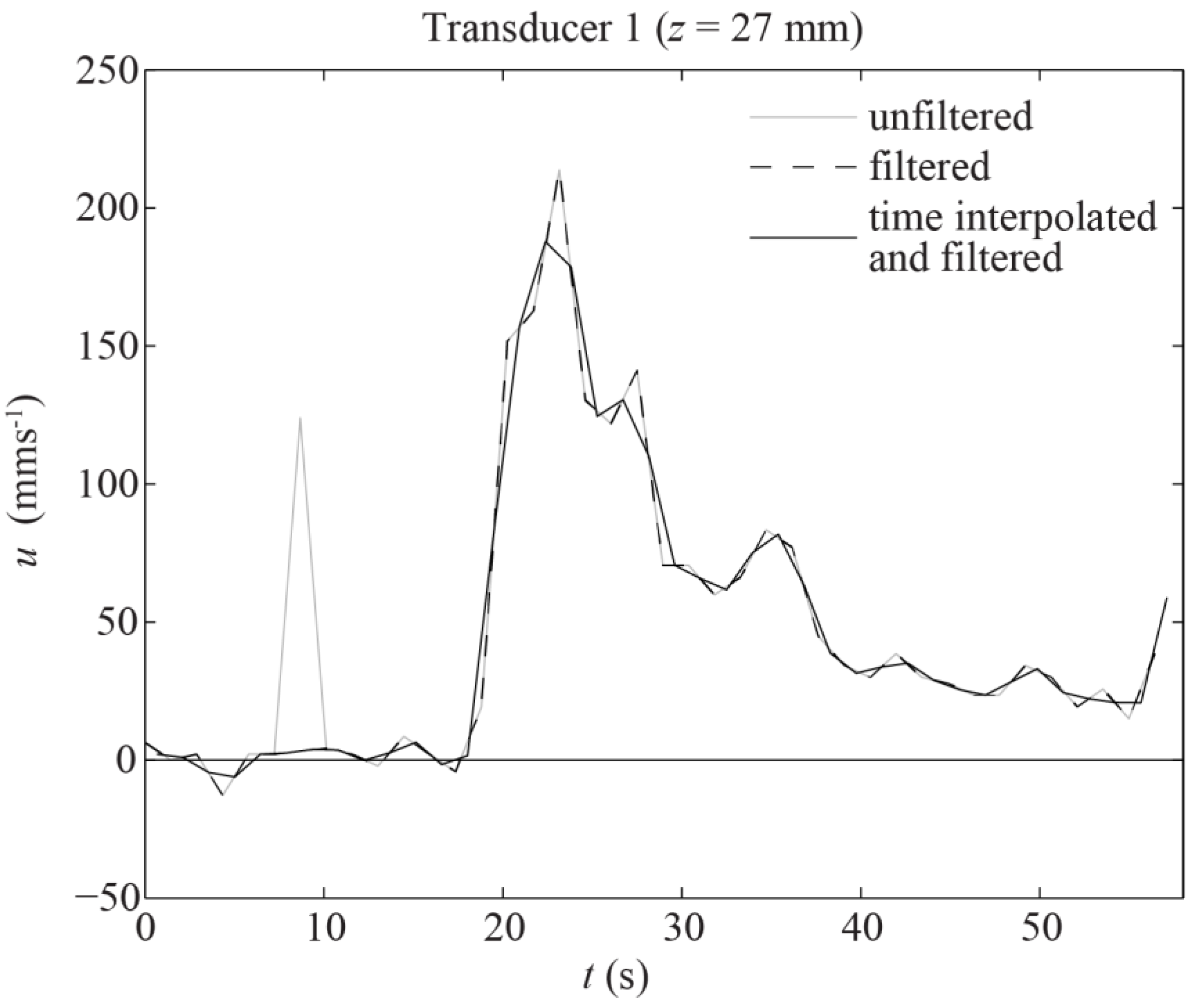
A piecewise cubic Hermite interpolation similar to [41] was applied to the velocity data as transducers cannot record simultaneously. For each full transducer cycle, an instantaneous velocity was interpolated for all channels at a time, t, equal to the average time in each cycle’s elapsed time range. Figure 5 shows the effectiveness of the data filtering. In this example, a time-series plot of velocity versus time for transducer #1 is shown for test NS. The velocities are those recorded from the 58th virtual channel of the transducer. A significant noise spike at approximately 9 s has been removed, whilst the time interpolation evidently smoothed the small fluctuations in velocity.
3.2. Photometric Data
Photometric analysis of the turbidity currents involved manipulation of the captured images to obtain flow progression contour plots by layering the outer boundaries of the propagating current for each image. In total, 80–110 frames of turbidity current evolution were obtained at 4.5 Hz for each test run. Frames captured were saved locally to the on-board camera memory, and subsequently uploaded to a computer for pre- and post-processing. Pre-processing of the frames for the removal of lens distortion using known calibration points, together with adjustment of brightness and contrast, was achieved using batch processing in Adobe Photoshop. The lens distortion and rotation correction settings were optimized for each test run to ensure that the basin sides aligned on a square grid. Thereafter, the frames were batch-cropped to the area of interest, converted to greyscale in MATLAB (the UVP rig assigned black), and transferred to a binary image with a threshold to ensure best identification of the turbidity outline. White pixels outside the turbidity current outline were removed, resulting in a final outline for each frame (Figure 6). For each test, all frame outlines were merged into a single plot showing the contoured, time-wise progression of the frontal current boundary.
4. Results and Discussion
For each obstacle configuration, the 10 cycles from when the turbidity current reached the analysis area (14.5 s in total) were used for the velocity analysis. This was based on [8], who used a time window of 10 s from when the current reached their analysis area. However, a slightly larger time window was applied for the present study as the UVP transducer read at a lower time resolution.
The transducer channels were divided into five spatial regions (Figure 7). The regions were based on [12], which divided the flow of turbidity currents over square cylinders into five regions: an approaching region; a region directly in front of the obstacle; a region directly above the obstacle; a region immediately after the obstacle; and a region further downstream of the obstacle. In the case of this study, one region was allocated before the obstacle, one above the obstacle, one directly after the obstacle, and two further downstream. These chosen regions were slightly different to [12], as they were adjusted to trends observed in the non-averaged intensity plots of each individual transducer.
4.1. Velocity Profile Development
The filtered horizontal velocities from each transducer were averaged for each region of interest, and subsequently plotted against height, non-dimensionalised by ambient water height, z0 (Figure 8). For practical reasons, transducer measurements could not be taken at the bed level, hence velocity at the bed was taken as 0 mm s−1, to reflect the no-slip boundary condition. A linear profile was fitted to interpolate between the data points.
umax was found to remain consistent in magnitude for all regions in test NS, with a mean of 108 mm s−1. As expected, the control test NS maintained the highest umax out of all scenarios due to the smooth bed and absence of the obstacle. umax was also found to be at a height of z/z0 ≈ 0.15–0.3, which agrees with the findings of [7]. The rough substrate (test NR) was found to reduce umax in all regions by a mean of 27%. u also shows a sharper vertical gradient above umax than smooth tests.
The velocity profiles of both obstacle tests (OS, OR) showed that the obstacle does not have a clear effect on reducing umax throughout the regions. Oehy et al. [26] showed that umax decreased by 50% over the obstacle, but their obstacle had a height of ≈0.27z0. The obstacle height in the present study (≈0.08 z0) is clearly not great enough to significantly influence umax. However, both obstacle tests show that umax occurs at a height of z/z0 = 0.15–0.2 above the obstacle, which was higher than non-obstructed tests. This was highlighted in region 4 above and immediately upstream of the obstacle, where flow prior to the obstacle was inhibited and directed over the obstacle. This was supported when reviewing spatial velocity contours of the current immediately after passing of the current head which showed small areas of zero velocity upstream of the obstacle (Figure 9). Oshaghi et al. [25] showed that the presence of an obstacle caused the velocity profile in regions prior to the obstacle to become distorted and in some cases, reduced umax. This was also evident in the experimental work of [43]. Similar to the present study, [43] showed that umax increases in height immediately prior to and above the obstacle. The overall inability of the obstacle to perceptibly reduce umax does not rule out the potential influence on sedimentation, however. Alexander and Morris [37] suggested that obstacles of a height much less than z1 are still likely to affect local sediment structures.
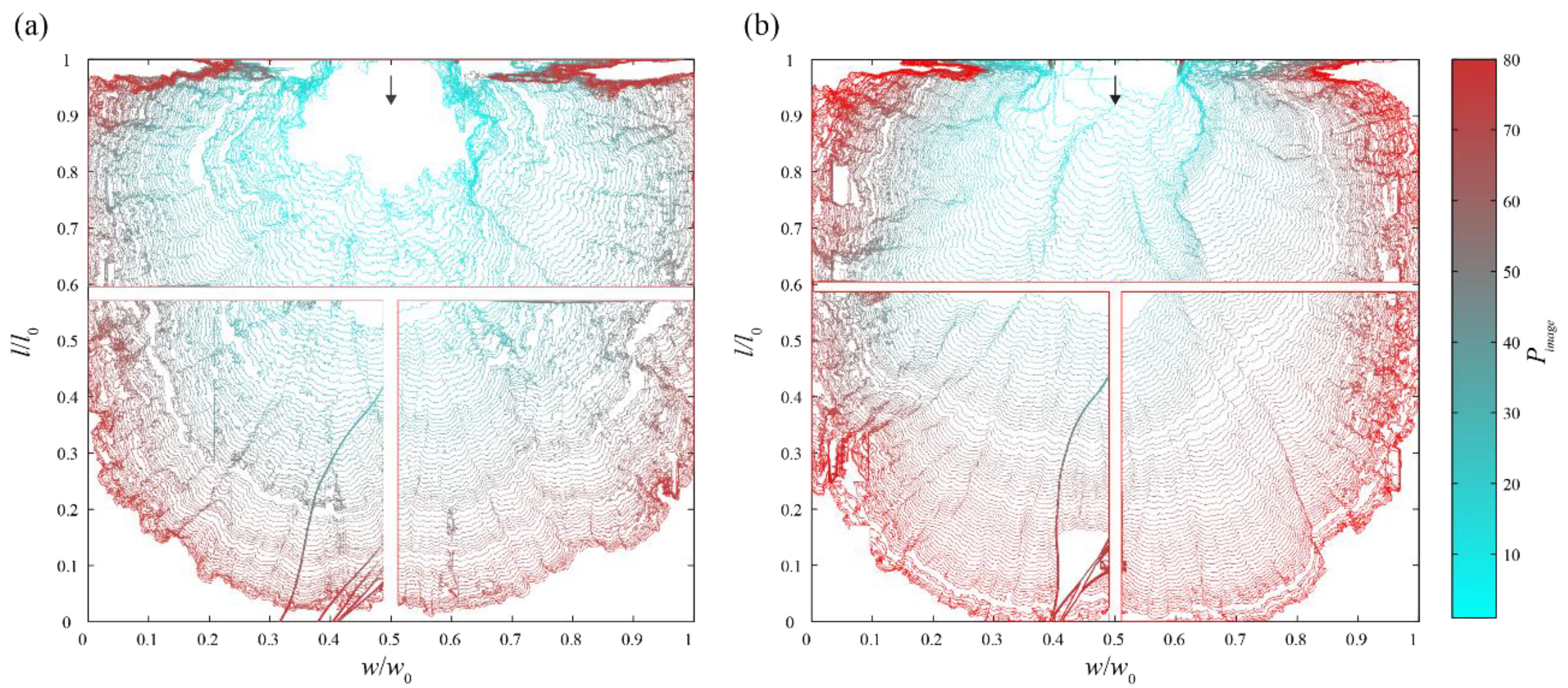
All tests tended to show weak negative velocities in the upper regions of the profiles, caused by the presence of a reverse ambient flow above the current. A reverse hydraulic bore reflected off the obstacle does not appear to be present in Figure 8. Such bores are common in studies where the obstacle is of a significant height [25,26,43]. Figure 9a shows that instantaneous reverse flows were present within the current head upon impact with the obstacle. This supports the presence of Kelvin-Helmholtz instabilities within the mixing layer between the current and ambient fluid, but cannot prove the presence of a hydraulic bore. Such phenomena were not present for test OR, suggesting that the rough bed inhibits the formation of Kelvin-Helmholtz instabilities immediately upstream of the obstacle. This is in agreement with [13], which observed less large-scale billows with an increase in basal roughness. Figure 10 shows that the current front, which expanded radially, had a well-defined head with large billows at the rear. In some areas, the head appeared to detach from the current body. Lobe and cleft structures at the current front appeared to group in similar-sized sub-radial protrusions; however, these became less apparent as the current progressed. In contrast, the head was visually less definable over a rough substrate, and sub-radial groupings of front instabilities were not as pronounced. The asymmetrical nature of test NR was likely due to the pouring procedure of the slurry (Figure 11b).
Similar observations were made from the spatial contour plots. Figure 11a shows the evolution of the turbidity current in test NS. The contours appear noisy and have many small inconsistencies, compared to that of configuration NR, which has smoother perimeter outlines (Figure 11b). Figure 11b also shows a reduction in progressive development and the paths of lobe-and-cleft formations appear more consistent, as do their radii. La Rocca et al, [35] showed that, for experimental tests of currents over a range of different substrate roughness heights (0.7–3.0 mm), the velocity reduction is minimal in the initial inertia-buoyancy phase, but significant in the latter buoyancy-bed friction phase. This is also clear in Figure 11b, where contour spacing decreases as the current propagates, signifying a reduction in velocity.
4.2. Turbulence Intensities
Turbulence intensity, I, was highlighted by [8] as a common method for comparing the turbulence of saline and sediment-laden gravity currents. Turbulence intensity can be represented as the standard deviation of each transducer channel velocity over time:
where uʹ is the difference between each individual velocity (u) and the mean velocity (ū), which was calculated using a moving time window of three cycles. The cycle showing the initial passing of the head was not included due to the sharp velocity increase, similar to [8], which omitted the first second after the front had passed.
Intensities for each channel of the horizontal transducers were calculated using Equations (1) and (2). The intensity data from each transducer was subsequently averaged for each region. It must be noted that [8] calculated intensities from vertical velocities using one vertical UVP transducer located at the flume bed, facing upwards. However, for this study, turbulence intensities were calculated with horizontal velocities from transducers #1–9 and plotted against their non-dimensional height for each region (Figure 12). A linear approximation was used to vertically interpolate between data points. The average intensity of all regions for test OS was 20.6 mm s−1, which is slightly lower than test NS. The intensity profile in region 5 follows a close relationship with NS; however, there is an apparent third, lower maximum located at z/z0 ≈ 0.15. Test OR also shows the presence of three maxima in region 5, implying that the obstacle is of influence. Both obstacle configurations revert to two maxima from region 4; a more conventional profile as shown by [8]. They also show larger vertical fluctuations in intensity, particularly region 3, which relates to the local regions of increased and decreased velocities around the obstacle. The average intensity for NR was much lower, at 14.8 mm s−1, whilst OR was 16.2 mm s−1. Except for the third maximum, NS and OS appear to show similar profile shapes through all regions. This further supports that the obstacle has little effect on the overall mean turbulence intensity profile. Eggenhuisen and McCaffrey [8] clearly showed that the lower boundary turbulence maximum has a greater intensity when the current traverses a rough substrate. No such characteristic could be immediately identified in this study; however, a lower boundary maximum may be present between the measurement range of transducer #1 and the bed. All configurations seemed to have similar readings in region 2, with only OR showing a secondary local maxima. However, upon reaching region 1, turbulence intensities for all configurations showed a large range, implying that the similarities shown in region 2 cannot be interpreted as all tests reaching a point of sustained homogeneity. Further tests at distances beyond region 1 are needed to confirm this.
4.3. Future Potential of the Coupled Approach
The novelty of this paper lies in the combination of the two techniques, which has several benefits. Firstly, coupled measurement allows for testing program times and resources to be reduced by removal of the need to repeat tests with the separate techniques. This also removes any error which may be introduced by comparing repeated tests. Secondly, the ability to obtain quantitative data on flow dynamics and compare these with visual features provides a clearer understanding on current mechanisms. The Kelvin-Helmholtz instabilities identified through UVP analysis were visualized through photometric data, where their spatial position and lateral extent could be recognized—a finding which would be difficult to achieve through UVP alone, unless a significant amount of UVP probes were installed in a grid formation throughout the basin. Such an approach would be costly and more intrusive on flow.
For this specific study, a coupled UVP and photometric flow instrumentation approach is shown to be valuable in gaining new insights into how unconfined turbidity currents interact with an obstacle and varying substrate—a growing and relevant research area. Specifically, for this study, the quantitative data obtained by UVP provided a detailed insight into the velocity and turbulence intensity profiles of the unconfined current, for the immediate regions surrounding an obstacle. The results show that the development of velocity and turbulence intensity profiles of an unconfined current, taken along the central basin streamline are, in general, similar to confined studies. However, incorporating a larger obstacle may have more implications for the lateral movement of the current upon interaction.
Furthermore, we have shown that there is a minimal effect of the obstacle on reducing net umax, whilst the rough substrate caused a significant reduction in umax. The apparent presence of three turbulence intensity maxima prior to and above the obstacle shows a deviation from conventional turbulence profiles of turbidity currents. However, these maxima cannot be confirmed without further research. This is due to the uncertainty introduced by the small number of measured samples over the 10-cycle timestep, where the current experiences unsteady flow. With present-day UVP technology, it is not possible to obtain velocity profiles from multiple transducers simultaneously without installing many processing consoles—a costly and impractical solution. Hence, the number of samples taken is limited by the time taken to cycle through all transducers and the net sampling time (14.5 s for the present study). A second future solution is to increase the net sampling time, which is recommended for quasi-steady turbidity current experiments—which have a steady flow compared to lock-exchange experiments. For lock-exchange experiments, further research is needed to set guidelines around a suitable cycle time/sampling time ratio.
The presence of negative velocities at the rear of the current head was found to relate well to the qualitative photometric data, where the radial extent of the current was visibly discernible from the current body. Finally, the spatial contours constructed from photometry provided valuable insight into the time and space-wise progressive development of instabilities within the current nose; particularly their lateral expansion.
The techniques presented are intended to be a starting point for future studies on unconfined turbidity flows. Improvements such as placing an additional camera on the side of the basin, combined with typical spatial calibration techniques [44,45,46], would allow for the quantification of photometric data. This would allow an investigation into common non-dimensional flow parameters, such as the entrainment parameter and Reynolds, Froude, and Richardson numbers, providing the scalability of laboratory-based results. Additionally, there is scope to install plan-view orientated cameras in confined environments to further investigate the common assumption that confined flow can be represented as two-dimensional.
5. Conclusions
By using a coupled UVP and photometric measurement approach, new data to study the effect of surface roughness on the propagation of turbidity currents is presented. It was found that the rough substrate reduces the turbidity current maximum velocity, umax, by a mean of 27% through the analysis area. The rough substrate also reduced the progressive development and subdivision of lobe-and-cleft formations, which was shown through both velocity profiles and spatial contours. A reduction in velocities immediately above and behind the obstacle, paired with a region of increased velocities downstream, suggested the obstacle had only minor effects on local velocities. A global reduction of intensities was evident with the introduction of a rough substrate; however, it did not appear to significantly change the intensity profile. The obstacle appeared to create three local turbulence intensity maxima upstream, which dissipated to two downstream; however, their presence cannot be confirmed without future research employing a lower UVP cycle time to net sample time ratio. Overall, the velocity and turbulence profiles were found to be similar in shape to typical unconfined current profiles.
The presence of Kelvin-Helmholtz instabilities was confirmed through both UVP and photometric analysis. We have shown how qualitative photometry can be used to strengthen findings from quantitative UVP data, by providing high visual detail of the current’s lateral progression and confirming the presence of lobe-and-cleft groups for the case of a smooth bed. Our synchronized measurement methodology opens new doors for better understanding the highly dynamic processes that occur during turbidity current propagation.
Author Contributions
R.I.W. and H.F. conceived and designed the study, obtained the experimental data, and wrote the paper. Wilson performed the bulk of the data analysis and wrote the first draft of the manuscript.
Funding
This research received no external funding.
Acknowledgments
The authors would like to thank the technical staff, Geoff Kirby and Jim Luo, for their valuable support. We would also like to thank Jenny McArthur, who assisted in the collection and processing of photometric data. Finally, we thank Craig Stevens for the fruitful discussions which have helped improve our understanding of the topic.
Conflicts of Interest
The authors declare no conflict of interest.
References
- Kneller, B.; Buckee, C. The structure and fluid mechanics of turbidity currents: A review of some recent studies and their geological implications. Sedimentology 2000, 47, 62–94. [Google Scholar] [CrossRef]
- Meiburg, E.; Kneller, B. Turbidity currents and their deposits. Annu. Rev. Fluid Mech. 2010, 42, 135–156. [Google Scholar] [CrossRef]
- Middleton, G.V. Sediment deposition from turbidity currents. Annu. Rev. Earth Planet. Sci. 1993, 21, 89–114. [Google Scholar] [CrossRef]
- Weimer, P.; Link, M.H. Global petroleum occurrences in submarine fans and turbidite systems. In Seismic Facies and Sedimentary Processes of Submarine Fans and Turbidite Systems; Weimer, P., Link, M.H., Eds.; Springer: New York, NY, USA, 1991; pp. 9–67. [Google Scholar]
- Felix, M.; Sturton, S.; Peakall, J. Combined measurements of velocity and concentration in experimental turbidity currents. Sediment. Geol. 2005, 179, 31–47. [Google Scholar] [CrossRef]
- Altinakar, M.S.; Graf, W.H.; Hopfinger, E.J. Flow structure in turbidity currents. J. Hydraul. Res. 1996, 34, 713–718. [Google Scholar] [CrossRef]
- Kneller, B.; Bennett, S.; McCaffrey, W.D. Velocity structure, turbulence and fluid stresses in experimental gravity currents. J. Geophys. Res. Oceans 1999, 104, 5381–5391. [Google Scholar] [CrossRef] [Green Version]
- Eggenhuisen, J.T.; McCaffrey, W.D. The vertical turbulence structure of experimental turbidity currents encountering basal obstructions: Implications for vertical suspended sediment distribution in non-equilibrium currents. Sedimentology 2012, 59, 1101–1120. [Google Scholar] [CrossRef]
- Nogueira, H.I.S.; Adduce, C.; Alves, E.; Franca, M.J. Dynamics of the head of gravity currents. Environ. Fluid Mech. 2014, 14, 519–540. [Google Scholar] [CrossRef]
- Gladstone, C.; Pritchard, D. Patterns of deposition from experimental turbidity currents with reversing buoyancy. Sedimentology 2010, 57, 53–84. [Google Scholar] [CrossRef] [Green Version]
- Heezen, B.C.; Ewing, M. Turbidity currents and submarine slumps, and 1929 grand banks earthquake. Am. J. Sci. 1952, 250, 849–873. [Google Scholar] [CrossRef]
- Gonzalez-Juez, E.; Meiburg, E.; Constantinescu, G. Gravity currents impinging on bottom-mounted square cylinders: Flow fields and associated forces. J. Fluid Mech. 2009, 631, 65–102. [Google Scholar] [CrossRef]
- Nogueira, H.I.S.; Adduce, C.; Alves, E.; Franca, M.J. Analysis of lock-exchange gravity currents over smooth and rough beds. J. Hydraul. Res. 2013, 51, 417–431. [Google Scholar] [CrossRef] [Green Version]
- Cenedese, C.; Nokes, R.; Hyatt, J. Lock-exchange gravity currents over rough bottoms. Environ. Fluid Mech. 2018, 18, 59–73. [Google Scholar] [CrossRef]
- Bursik, M.I.; Woods, A.W. The effects of topography on sedimentation from particle-laden turbulent density currents. J. Sediment. Res. 2000, 70, 53–63. [Google Scholar] [CrossRef]
- Nasr-Azadani, M.M.; Meiburg, E. Turbidity currents interacting with three-dimensional seafloor topography. J. Fluid Mech. 2014, 745, 409–443. [Google Scholar] [CrossRef]
- Lane-Serff, G.F.; Beal, L.M.; Hadfield, T.D. Gravity current flow over obstacles. J. Fluid Mech. 1995, 292, 39–53. [Google Scholar] [CrossRef]
- Rottman, J.W.; Simpson, J.E.; Hunt, J.C.R.; Britter, R.E. Unsteady gravity current flows over obstacles: Some observations and analysis related to the phase ii trials. J. Hazard. Mater. 1985, 11, 325–340. [Google Scholar] [CrossRef]
- Asghari Pari, S.A.; Kashefipour, S.M.; Ghomeshi, M. An experimental study to determine the obstacle height required for the control of subcritical and supercritical gravity currents. Eur. J. Environ. Civ. Eng. 2017, 21, 1080–1092. [Google Scholar] [CrossRef]
- Ermanyuk, E.; Gavrilov, N. Interaction of internal gravity current with an obstacle on the channel bottom. J. Appl. Mech. Tech. Phys. 2005, 46, 489–495. [Google Scholar] [CrossRef]
- Ermanyuk, E.; Gavrilov, N. Interaction of an internal gravity current with a submerged circular cylinder. J. Appl. Mech. Tech. Phys. 2005, 46, 216–223. [Google Scholar] [CrossRef]
- Gonzalez-Juez, E.; Constantinescu, G.; Meiburg, E. A study of the interaction of a gravity current with a square cylinder using two-dimensional numerical simulations. In Proceedings of the 26th International Conference on Offshore Mechanics and Arctic Engineering, San Diego, CA, USA, 10–15 June 2017; ASME: San Diego, CA, USA, 2007; Volume 2007, pp. 861–870. [Google Scholar]
- Gonzalez-Juez, E.; Meiburg, E. Shallow-water analysis of gravity-current flows past isolated obstacles. J. Fluid Mech. 2009, 635, 415–438. [Google Scholar] [CrossRef]
- Tokyay, T.; Constantinescu, G. The effects of a submerged non-erodible triangular obstacle on bottom propagating gravity currents. Phys. Fluids 2015, 27, 056601. [Google Scholar] [CrossRef]
- Oshaghi, M.R.; Afshin, H.; Firoozabadi, B. Experimental investigation of the effect of obstacles on the behavior of turbidity currents. Can. J. Civ. Eng. 2013, 40, 343–352. [Google Scholar] [CrossRef]
- Oehy, C.; Schleiss, A.J. Control of turbidity currents in reservoirs by solid and permeable obstacles. J. Hydraul. Eng. 2007, 133, 637–648. [Google Scholar] [CrossRef]
- Janocko, M.; Cartigny, M.; Nemec, W.; Hansen, E. Turbidity current hydraulics and sediment deposition in erodible sinuous channels: Laboratory experiments and numerical simulations. Mar. Pet. Geol. 2013, 41, 222–249. [Google Scholar] [CrossRef]
- Stagnaro, M.; Bolla Pittaluga, M. Velocity and concentration profiles of saline and turbidity currents flowing in a straight channel under quasi-uniform conditions. Earth Surf. Dyn. 2014, 2, 167–180. [Google Scholar] [CrossRef] [Green Version]
- Chowdhury, M.R.; Testik, F.Y. Laboratory testing of mathematical models for high-concentration fluid mud turbidity currents. Ocean Eng. 2011, 38, 256–270. [Google Scholar] [CrossRef]
- Jacobson, M.R.; Testik, F.Y. Turbulent entrainment into fluid mud gravity currents. Environ. Fluid Mech. 2014, 14, 541–563. [Google Scholar] [CrossRef]
- Hallworth, M.A.; Huppert, H.E.; Phillips, J.C.; Sparks, R.S.J. Entrainment into two-dimensional and axisymmetric turbulent gravity currents. J. Fluid Mech. 1996, 308, 289–311. [Google Scholar] [CrossRef]
- Marleau, L.J.; Flynn, M.R.; Sutherland, B.R. Gravity currents propagating up a slope in a two-layer fluid. Phys. Fluids 2015, 27, 036601. [Google Scholar] [CrossRef]
- Mirajkar, H.N.; Tirodkar, S.; Balasubramanian, S. Experimental study on growth and spread of dispersed particle-laden plume in a linearly stratified environment. Environ. Fluid Mech. 2015, 1241–1262. [Google Scholar] [CrossRef]
- Choi, S.-U.; Garcia, M.H. Spreading of gravity plumes on an incline. Coast. Eng. J. 2001, 43, 221. [Google Scholar] [CrossRef]
- La Rocca, M.; Adduce, C.; Sciortino, G.; Pinzon, A.B. Experimental and numerical simulation of three-dimensional gravity currents on smooth and rough bottom. Phys. Fluids 2008, 20, 106603. [Google Scholar] [CrossRef]
- Sahuri, R.M.; Kaminski, A.K.; Flynn, M.R.; Ungarish, M. Axisymmetric gravity currents in two-layer density-stratified media. Environ. Fluid Mech. 2015, 15, 1035–1051. [Google Scholar] [CrossRef]
- Alexander, J.; Morris, S.A. Observations on experimental, nonchannelized, high-concentration turbidity currents and variations in deposits around obstacles. J. Sediment. Res. 1994, 64, 899–909. [Google Scholar]
- Morris, S.A.; Alexander, J. Changes in flow direction at a point caused by obstacles during passage of a density current. J. Sediment. Res. 2003, 73, 621–629. [Google Scholar] [CrossRef]
- Choux, C.M.A.; Baas, J.H.; McCaffrey, W.D.; Haughton, P.D.W. Comparison of spatio-temporal evolution of experimental particulate gravity flows at two different initial concentrations, based on velocity, grain size and density data. Sediment. Geol. 2005, 179, 49–69. [Google Scholar] [CrossRef]
- Gray, T.E.; Alexander, J.; Leeder, M.R. Longitudinal flow evolution and turbulence structure of dynamically similar, sustained, saline density and turbidity currents. J. Geophys. Res. 2006, 111, C08015. [Google Scholar] [CrossRef]
- Gray, T.E.; Alexander, J.; Leeder, M.R. Quantifying velocity and turbulence structure in depositing sustained turbidity currents across breaks in slope. Sedimentology 2005, 52, 467–488. [Google Scholar] [CrossRef]
- Keevil, G.M.; Peakall, J.; Best, J.L.; Amos, K.J. Flow structure in sinuous submarine channels: Velocity and turbulence structure of an experimental submarine channel. Mar. Geol. 2006, 229, 241–257. [Google Scholar] [CrossRef]
- Sequeiros, O.E.; Spinewine, B.; Garcia, M.H.; Beaubouef, R.T.; Sun, T.; Parker, G. Experiments on wedge-shaped deep sea sedimentary deposits in minibasins and/or on channel levees emplaced by turbidity currents. Part I. Documentation of the flow. J. Sediment. Res. 2009, 79, 593–607. [Google Scholar] [CrossRef]
- Jacobson, M.R.; Testik, F.Y. On the concentration structure of high-concentration constant-volume fluid mud gravity currents. Phys. Fluids 2013, 25, 016602. [Google Scholar] [CrossRef]
- Nogueira, H.I.S.; Adduce, C.; Alves, E.; Franca, M.J. Image analysis technique applied to lock-exchange gravity currents. Meas. Sci. Technol. 2013, 24, 047001. [Google Scholar] [CrossRef] [Green Version]
- Wilson, R.I.; Friedrich, H.; Stevens, C. Image thresholding process for combining photometry with intrusive flow instruments. J. Hydraul. Res. 2018, 56, 282–290. [Google Scholar] [CrossRef]
Figure 1.
Typical velocity profile of an unobstructed gravity current, where velocity within the lower wall region represents a logarithmic shape and velocity in the upper jet region represents a Gaussian shape.
Figure 1.
Typical velocity profile of an unobstructed gravity current, where velocity within the lower wall region represents a logarithmic shape and velocity in the upper jet region represents a Gaussian shape.

Figure 2.
(a) Schematic plan view of the laboratory basin, including the location of the square cylindrical obstacle and false floor; (b) Illumination and lock-box configuration within the basin.
Figure 2.
(a) Schematic plan view of the laboratory basin, including the location of the square cylindrical obstacle and false floor; (b) Illumination and lock-box configuration within the basin.

Figure 3.
Grainsize distribution of the kaolinite clay and Ballotini spherical glass beads, the sedimentary compounds used to create the turbidity current slurry.
Figure 3.
Grainsize distribution of the kaolinite clay and Ballotini spherical glass beads, the sedimentary compounds used to create the turbidity current slurry.

Figure 4.
Elevation view of the unconfined basin, showing the UVP transducer configuration (labelled transducer #1–14, clockwise from bottom) and area of analysis, including the position of the square obstacle.
Figure 4.
Elevation view of the unconfined basin, showing the UVP transducer configuration (labelled transducer #1–14, clockwise from bottom) and area of analysis, including the position of the square obstacle.

Figure 5.
Time-series plot of velocities for channel 58 of transducer #1, comparing the unfiltered, raw data to filtered (with a standard deviation filter) and a combination of filtered/time interpolated data.
Figure 5.
Time-series plot of velocities for channel 58 of transducer #1, comparing the unfiltered, raw data to filtered (with a standard deviation filter) and a combination of filtered/time interpolated data.

Figure 6.
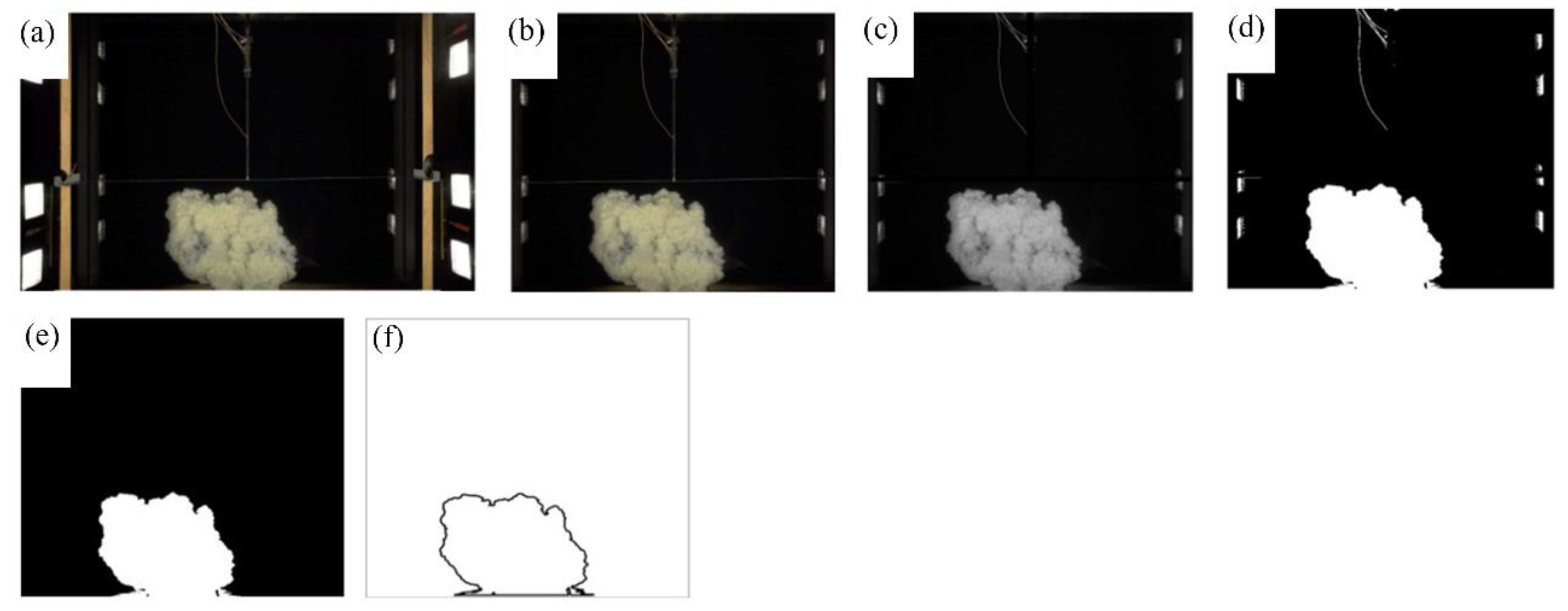
Step-by-step plan view of photometric image processing: (a) raw image; (b) cropped image adjusted for lens distortion; (c) greyscale conversion; (d) binary conversion; (e) removal of noise induced by the halogen lamps and UVP rack; and (f) delineated current boundary.
Figure 6.
Step-by-step plan view of photometric image processing: (a) raw image; (b) cropped image adjusted for lens distortion; (c) greyscale conversion; (d) binary conversion; (e) removal of noise induced by the halogen lamps and UVP rack; and (f) delineated current boundary.

Figure 7.
Elevation view of the five regions within the analysis area used for the velocity and turbulence intensity profile analysis. The regions were based on [12], with region widths optimized according to visible trends in non-averaged turbulence intensity plots.
Figure 7.
Elevation view of the five regions within the analysis area used for the velocity and turbulence intensity profile analysis. The regions were based on [12], with region widths optimized according to visible trends in non-averaged turbulence intensity plots.

Figure 8.
Non-dimensionalised vertical profiles of the horizontal velocity (u) of all obstacle configurations for each allocated region of interest, where u has been averaged, per region, for each transducer.
Figure 8.
Non-dimensionalised vertical profiles of the horizontal velocity (u) of all obstacle configurations for each allocated region of interest, where u has been averaged, per region, for each transducer.

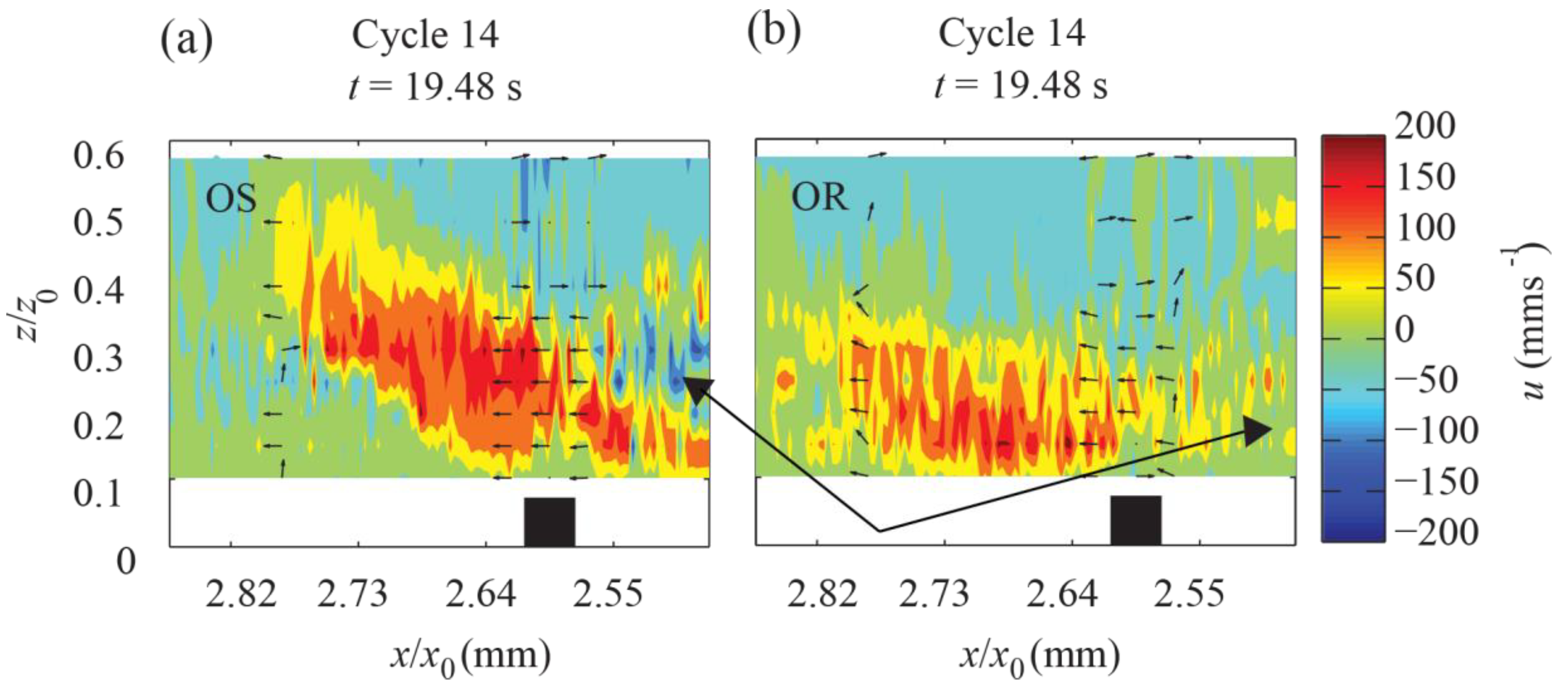
Figure 9.
Non-dimensionalised spatial velocity contour plots (obtained from UVP) comparing the arrival of the current head in the analysis area for both smooth (a) and rough (b) bed conditions. The current head is characterized by a forward velocity below a faint ambient reverse flow. Regions of reverse flow are present directly behind the head for test OS but not OR.

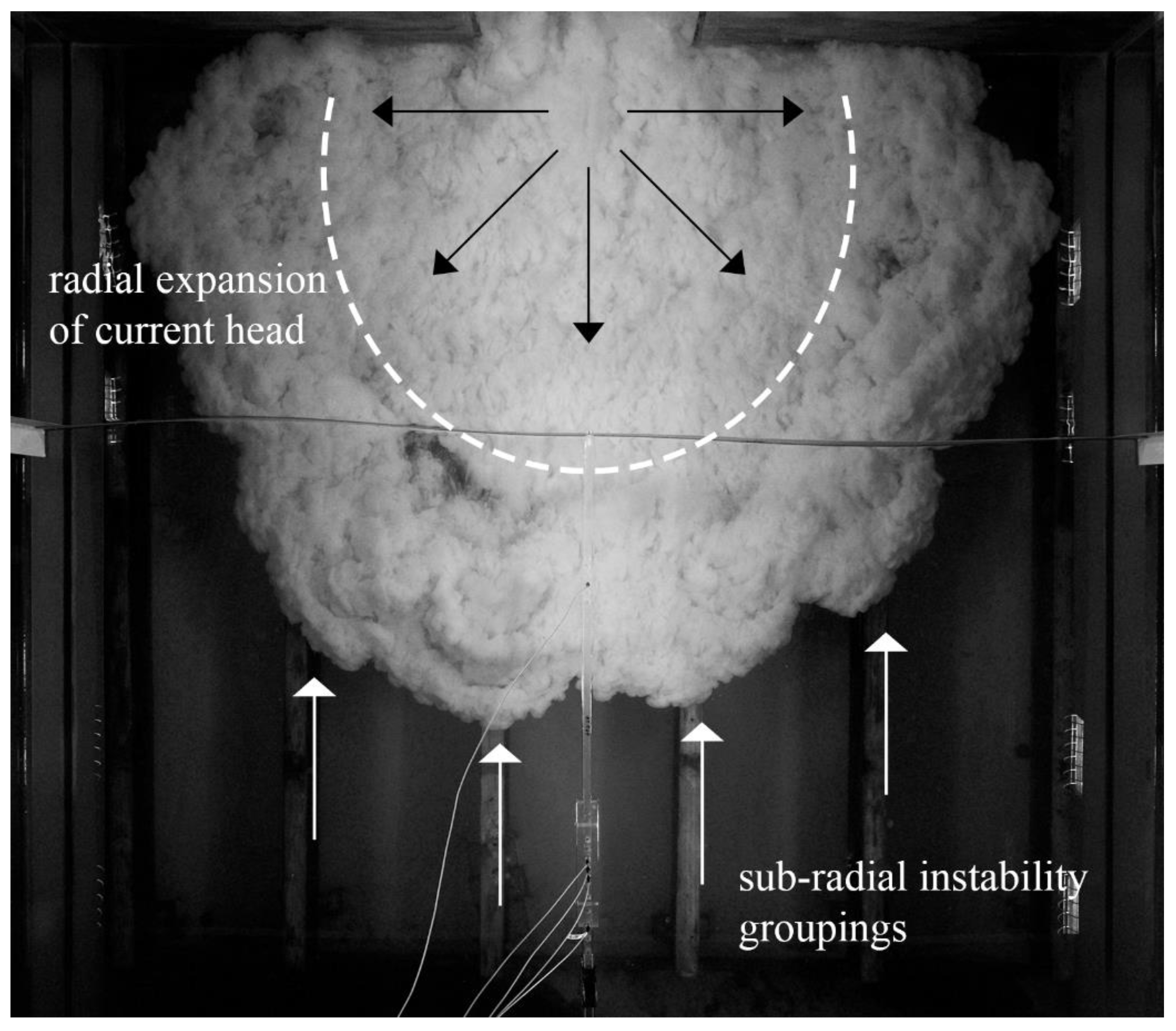
Figure 10.
Example plan images of the current in test NS. The unconfined nature of the basin causes the current to expand in a radial movement upon release. The current head appears well-defined, where it is seen to detach from the current body in various locations. Current front intensities are also seen to form sub-radial groups for a smooth bed.

Figure 11.
Spatially non-dimensionalised plan velocity contour plots from photometric analysis showing the progression of the current over the smooth substrate (a) and rough substrate (b). l0 and w0 represent the length and width of the image analysis area, respectively. Pimage represents the consecutive image number recorded after opening of the lock-box. The black arrows signify flow direction.

Figure 12.
Non-dimensionalised vertical profiles of the horizontal turbulence intensity (I) of all obstacle configurations for each allocated region of interest.
Figure 12.
Non-dimensionalised vertical profiles of the horizontal turbulence intensity (I) of all obstacle configurations for each allocated region of interest.


Table 1.
Transducer positioning.
| Transducer # | x/x0 | z/z0 | Transducer # | x/x0 | z/z0 |
|---|---|---|---|---|---|
| 1 | 2.91 | 0.10 | 8 | 2.91 | 0.48 |
| 2 | 2.91 | 0.15 | 9 | 2.91 | 0.57 |
| 3 | 2.91 | 0.20 | 10 | 2.78 | 0.94 |
| 4 | 2.91 | 0.24 | 11 | 2.63 | 0.94 |
| 5 | 2.91 | 0.29 | 12 | 2.60 | 0.94 |
| 6 | 2.91 | 0.34 | 13 | 2.57 | 0.94 |
| 7 | 2.91 | 0.38 | 14 | 1.73 | 0.94 |
Table 2.
UVP and camera parameters.
| Met-Flow UVP-DUO | |
| Sampling frequency (MHz) | 4 |
| Number of Bins | 128 |
| Bin width (mm) | 1.48 |
| Distance between bin centres (mm) | 1.67 |
| Measurement window (mm) | 25.9–237.36 |
| Speed of sound (ms−1) | 1480 |
| Velocity resolution (mms−1) | 2.138 |
| Velocity bandwidth (mms−1) | 547.3 |
| Cycles per pulse | 8 |
| Repetitions per profile | 32 |
| Sampling period (ms) | 15 |
| Full cycle time (s) | 1.45 |
| RF gain—US voltage (V) | 90 |
| Nikon D90 | |
| Lens | AF-S DX NIKKOR 18–105 mm |
| Camera mode | Manual |
| Capture mode | Continuous high-speed |
| Frame Rate (Hz) | 4.5 |
| Distance from free surface (m) | 2.045 |
| Shutter speed (s) | 1/200 |
| Aperture | f/3.5 |
| ISO | 200 |
| Image resolution (pixels) | 4288 × 2848 |
© 2018 by the authors. Licensee MDPI, Basel, Switzerland. This article is an open access article distributed under the terms and conditions of the Creative Commons Attribution (CC BY) license (http://creativecommons.org/licenses/by/4.0/).
Share and Cite
MDPI and ACS Style
Wilson, R.I.; Friedrich, H. Coupling of Ultrasonic and Photometric Techniques for Synchronous Measurements of Unconfined Turbidity Currents. Water 2018, 10, 1246. https://doi.org/10.3390/w10091246
AMA Style
Wilson RI, Friedrich H. Coupling of Ultrasonic and Photometric Techniques for Synchronous Measurements of Unconfined Turbidity Currents. Water. 2018; 10(9):1246. https://doi.org/10.3390/w10091246
Chicago/Turabian StyleWilson, Richard I., and Heide Friedrich. 2018. "Coupling of Ultrasonic and Photometric Techniques for Synchronous Measurements of Unconfined Turbidity Currents" Water 10, no. 9: 1246. https://doi.org/10.3390/w10091246
Note that from the first issue of 2016, this journal uses article numbers instead of page numbers. See further details here.