A Novel Methodology for Multiple-Year Regulation of Reservoir Active Storage Capacity


1
Environmental Engineering Laboratory, Department of Civil Engineering, University of Patras, 265 04 Patras, Greece
2
Hydraulic Engineering Laboratory, Department of Civil Engineering, University of Patras, 265 04 Patras, Greece
*
Author to whom correspondence should be addressed.
Water 2018, 10(9), 1254; https://doi.org/10.3390/w10091254
Submission received: 4 August 2018
/
Revised: 31 August 2018
/
Accepted: 12 September 2018
/
Published: 14 September 2018
(This article belongs to the Section Water Resources Management, Policy and Governance)
Abstract
:Reservoir design entails the determination of the required storage capacity over multiple years of low flow conditions to ensure the coverage of multiple-purpose water demands. Dam operation depends on many factors that may result in the decrease of required safe yields, leading to inadequate outflow supplies in the design period. This study addresses two issues: (a) the computation of reservoir active storage capacity performed with the aid of the new concept of a zero-height dam, a procedure easy to interpret physically and implement computationally; and (b) the generation of appropriate inflow data, provided that a substantial record of monthly inflows is available. The treatment of the inflow data for the generation of inflow sequences for any desired regulation period is performed by two original methods (First and Second), which are entirely different from other available methods and allow for the selection of a reservoir capacity with the desired level of exceedance probability. The two methods proposed give practically the same results. However, the Second Method, which generates inflow data consisting of hydrologic years with inflow values for each month randomly selected from the observed values for that month, is superior in terms of the ease with which inflow sequences are generated. Also, due to the large size of the random sample that can be generated, the exceedance probability curves are very smooth and allow for the easy selection of reservoir storage capacity with any level of desired exceedance probability. The proposed methodology may be useful for consultants and reservoir managers.
1. Introduction
The design of a reservoir project entails the determination of the required storage capacity over multiple years of low flow conditions to ensure the coverage of multiple-purpose water demands. Water storage during water-rich seasons and its use during dry seasons have occupied man since ancient times. The oldest dam, called Sadd el-Kafara, was constructed around 2950–2750 B.C. by ancient Egyptians, but it failed after a few years [1]. The oldest operational dam of the world is the Quatinah Barrage of Lake Homs Dam in Syria, built between 1319–1304 B.C., during the reign of the Egyptian Pharaoh Sethi [2]. In our days there are in operation more than 14,500 dams worldwide [3]; their operation intervenes with the ecology of the area both positively and negatively. A sensitivity analysis showed that smaller reservoirs have substantial impacts on the spatial extent of flow alterations despite their minor role in total reservoir capacity [4]. Furthermore, dam operation depends on many factors that may result in the decrease of required safe yields, leading to inadequate outflow supplies in the design period. Such factors are: (a) increases in water demand due to increases in population (drinking water supplies) or due to increases in irrigation demands, (b) increases in demand related to environmental standards such as maintaining downstream minimum releases for the in-stream protection of aquatic habitats, (c) future declining trends of inflows due to climatic changes, and (d) loss of reservoir capacity and yield due to sedimentation. The factors (a), (b), and (c) can be incorporated in the procedure that will be described in the present work while factor (d) is not incorporated, since we aim to determine active storage capacity.
The complexity of reservoir active capacity design depends on the type of flow regulation. Typically, monthly stream flows are utilized, although shorter or longer periods can also be used. Furthermore, the period of flow regulation is critical, i.e., the number of low-flow years for which the reservoir will be designed. One, however, must be aware of the fact that the design must be optimized in terms of the relation between yield versus cost and in that respect design inflows must satisfy some predetermined level of probability of occurrence. Thus, the design entails two major components:
- Determination of yearly inflow values, which will provide the desired regulation with a predetermined level of probability of occurrence, and
- Reservoir capacity determination based on the maximum absolute cumulative deficit of water, which must be stored during monthly water surplus periods to allow for the coverage of demand during deficit months.
The latter has historically evolved from the procedure initially proposed by Rippl [5] and subsequently modified by various investigators (e.g., [6,7]). In the following, a variation of the method based on the new concept of a zero-height dam will be presented and used.
The determination of the sequence of low-flow yearly rates and their corresponding monthly inflow values that will be used in the computation of reservoir storage capacity has been addressed extensively in the literature. Clark et al. [8] have addressed the problem, and an extensive review has been presented more recently in the Hydrology Handbook [6].
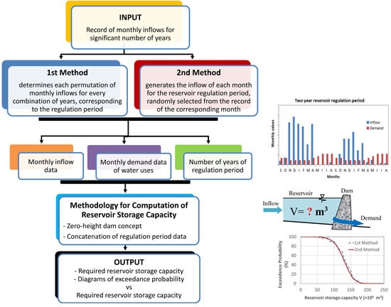
In the present study an altogether different approach will be presented. The present approach (see Section 3—Inflow and Demand Data) is considered valid for cases where a substantial record of yearly flow rates and their corresponding monthly values are available. For the given demands, the proposed approach generates as many as possible numbers of probable scenarios of yearly series (1 to 10 years) for the desired regulation periods, based on recorded monthly inflows. For each scenario the required reservoir storage capacity was calculated using the zero-height dam concept (see Section 2) and the results are shown in diagrams as probability (%) versus required reservoir storage capacity.
The objective of this study is twofold: (a) to present a method for the computation of reservoir active storage capacity, which is easier to interpret physically and implement computationally, and (b) to describe and implement an approach for the generation of a sequence of inflow data, for the desired period of reservoir regulation, from an available record of substantial length.
The proposed approach may be useful for engineers, other scientists, decision-makers, and authorities involved in the consultation and management of reservoirs.
2. The Concept of Zero-Height Dam
The most significant characteristic of a reservoir is its storage capacity, which in turn determines its yield. Yield is defined as the volume of water that can be supplied during a specified period. Provided that the sequence of, say, monthly inflow rates, Qin, has been selected and the sequence of monthly demand rates, Qd, has been prescribed, then the cumulative inflow volume, Vin, and the cumulative demand volume from an initial time, t1, up to a desired time, t, will be given by the relationships:
The difference between Vin and Vd will be given by the relationship:
where ΔV is the cumulative net inflow volume.
It is obvious that the derivative of ΔV is equal to the difference between Qin and Qd, i.e.,:
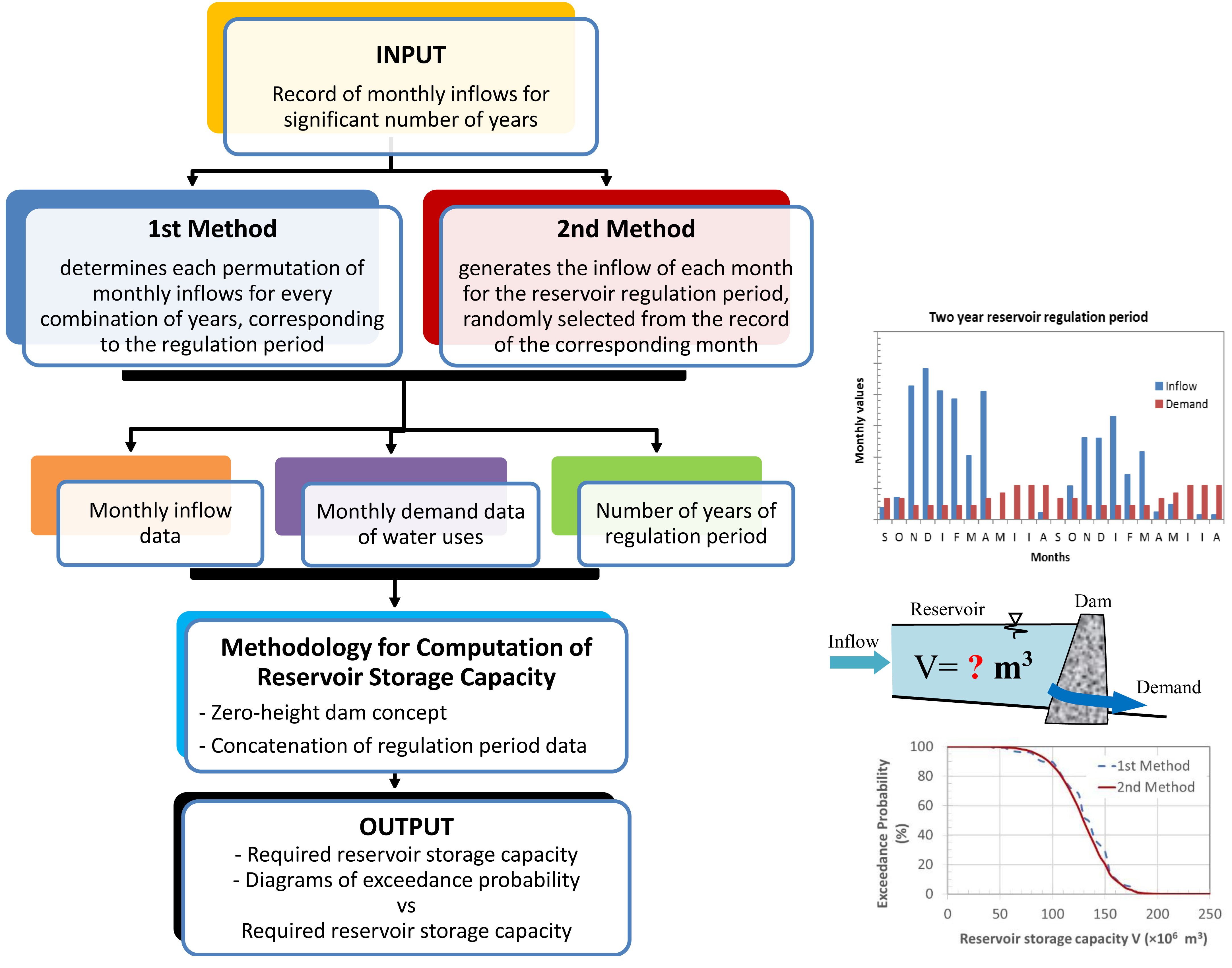
From Equation (4) it follows that, when Qin (t) = Qd (t), the cumulative inflow volume, ΔV, (see Equation (3)) will have a local maximum or minimum value. More specifically, when Equation (4) has a negative derivative at Qin (t) = Qd (t), then ΔV has a local maximum value, and vice versa. Consequently, there exists at least one negative local minimum or at least one positive local maximum within the time interval under consideration when the derivative of Equation (4) is, respectively, negative or positive at the initial point of the time interval. This implies that there will be a water deficit in the interval with a negative minimum, which will be covered by the water stored in the reservoir. On the other hand, there will be a water surplus in the interval with a positive maximum; this surplus will be, partially or fully, stored in the reservoir to cover deficits. The above information is schematically shown in Figure 1.
According to the preceding mathematical formulation, the procedure for the determination of the minimum storage capacity of a reservoir for multiple-year regulation is as follows. The hydrograph of the difference between inflow and demand rates is constructed, as shown in Figure 1. This hydrograph contains the information regarding the points at which Qin (t) = Qd (t), hence the points at which Equation (4) becomes zero, and the intervals between successive equality between values of Qin (t) and Qd (t) where there is a surplus or deficit of water. The cumulative net inflow volume is computed from Equation (3) for t = t2, with t1, t2 being the successive times at which Qin (t) = Qd (t) (see Equation (4) and Figure 1). The cumulative net inflow volume for the interval t1 to t2 can be computed from Equation (3). A shortcoming of this approach relates to the initial storage in the reservoir. To address the problem, Thomas and Fiering [9] introduced the Sequent Peak Algorithm, in which the analysis is performed with the selected record, for multiple-year regulation, concatenated with itself. This approach provides safe results when the total net cumulative inflow volume, ΔVT, is greater or equal to zero, where:
and T is the regulation period. On the other hand, the concatenation of the multiple-year record with itself will not provide the required storage capacity when ΔVT < 0, because the required volume will keep increasing if we concatenate the record one more time. This may be interpreted either as a poor choice of the site for the required demands or, more realistically, that the probability of appearance of the selected inflow data for more than two regulation periods in a row is negligible. In the latter case, it would be safe to accept the required storage capacity obtained from two regulation periods. Based on the above, we define as the minimum required active storage capacity the largest deficit computed during a period equal to twice the reservoir regulation period, as per the concept of the Sequent Peak Algorithm. This implies that the reservoir will have an active volume of water equal to zero at least once during the computation period.
Application of the aforesaid methodology is based on the concept of a zero-height dam, which is being introduced for the first time in the present study. The way that the concept of a zero-height dam works is as follows: at the location where the dam is to be built, we assume that there exists a hypothetical dam of zero height which performs the following tasks: (a) records the inflow volume and demand volume for each time interval of the concatenated regulation period and computes the difference between them, (b) when the difference is negative there is a water volume deficit, while there is a surplus of water volume when the difference is positive, (c) computes the cumulative volume deficit for all successive time intervals, (d) during the computation of the cumulative volume deficit, if this becomes positive (which means that there exists a surplus of water) the cumulative deficit (i.e., surplus) is set equal to zero since a zero-height dam cannot store any water, and (e) defines the largest absolute value of the cumulative volume deficits (which appear after intervals where the deficit is zero) as the required storage capacity of the reservoir.
This methodology is illustrated in the following three examples, in which a three-year regulation period of a proposed reservoir is examined, with the time interval of the required information for demand and the selected information for inflow being equal to one year. The information is concatenated with itself and the computations are summarized in Table 1, Table 2 and Table 3 for VT > 0, VT = 0, and VT < 0, respectively.
From Table 1, Table 2 and Table 3, one can observe that as VT decreases, the required storage, computed with the concatenation of data—as suggested by the Sequent Peak Algorithm—increases. More interesting is the case of VT < 0, where the record concatenated with itself twice gives even higher reservoir capacity in the third repeat of the cycle. This is shown only for information purposes, because the repeat of the cycle three times in a row may be considered highly unlikely. In Table A2 of Appendix A we present another example, in which a one-year regulation period of a proposed reservoir is examined with the time interval of the required information for demand and the selected information for inflow being equal to one month.
3. Inflow and Demand Data
3.1. Site Information and Demand Data
Except for the concept of the zero-height dam, the other main thrust of this paper is on the methodology for the generation of inflow data. Nevertheless, basic information on the site and a set of specific data for downstream demands are also given, to highlight the manner in which the two main components of the present study (i.e., the concept of the zero-height dam and the methodology of generating inflow data) can be applied for the computation of reservoir active storage capacity.
The hydrologic basin upstream of the dam site under investigation is in North Western Peloponnisos, Greece, with an area of 1000 km2. Actual discharge measurements are not available, but a time-series of monthly precipitation heights is available for the period of September 1974 to August 1995. These data have been collected near the hypothetical dam site. The precipitation data are given in Table A1 of Appendix A. It must be noted that neither the hydrology of the area nor the demand of water affects the applicability of the methodology proposed herein. Also, for analysis purposes, it is assumed that the surface run-off coefficient is equal to unity. Thus, the monthly precipitation data can be converted to inflow data (m3/month) for the proposed dam site after multiplication with 10−3 × 1000 × 10002 = 106.
Based on a preliminary investigation, it was determined that the demand must cover: (a) summer irrigation needs for 15,000 ha with an average monthly consumption of 2000 m3/ha, i.e., 30 × 106 m3/month, 50% of the summer consumption for April, May, September, and October, and 0% during the remaining months, (b) water supply for an urban area of 500,000 residents with mean daily consumption of 0.25 m3 per capita, i.e., 500,000 × 0.25 × 30 = 3.75 × 10⁶ m3/month during the summer months and 50% of the above (i.e., 1.875 × 10⁶ m3/month) during the rest of the year, and (c) demand for hydro-power generation, which was estimated to be 8.224 × 10⁶ m3/month. The temporal distribution of the demands is given in Table 4. It is noted that the specific values utilized herein can be covered by the flow rates even during the driest year of the available record.
3.2. Generation of Inflow Data
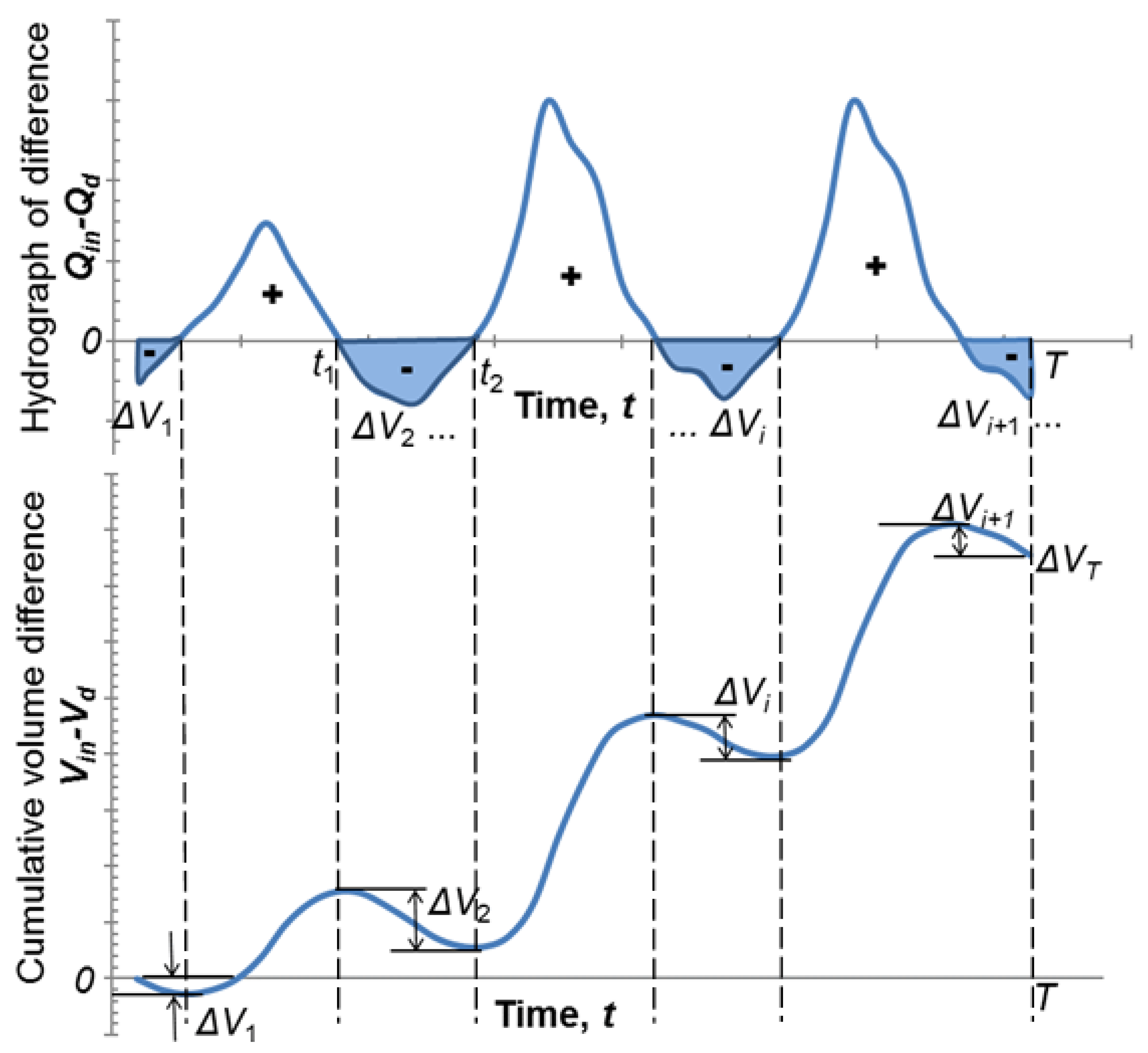
The stochastic generation of flow data has been the subject of intense investigation in the past (e.g., [9,10,11,12]). However, preliminary computations of required storage capacity for the available 21-year record revealed some interesting results, e.g., the computations shown in Table A2 of Appendix A produced a required storage capacity of 127.43 × 10⁶ m3 for a yearly inflow of 276.81 × 10⁶ m3, corresponding to the year 1991–1992. On the other hand, the required storage capacity for the year 1984–1985 was equal to 191.14 × 10⁶ m3, while the yearly inflow was 722.17 × 10⁶ m3. This implies that it is the monthly variations that primarily determine required storage capacity, and to a lesser extent the yearly values. Using the data from the 21 years of record, the computation of storage capacity for 1-year regulation did not reveal any correlation between storage capacity and yearly inflows or their important statistics, i.e., normalized standard deviation, skewness, and kurtosis. The results are shown in Figure 2.
Hence, in this paper, a different approach was employed, especially in view of the fact that we seek to determine storage capacity for multi-year regulation. Thus, the generation of inflow data from the available record was performed using two different methods.
In the first method (hereafter called the First Method) we employed the following procedure:
- We utilized the annual precipitation heights of the 21 hydrologic years and computed the average precipitation height for the combination of the 21 years per 1, 2, 3, 4, 5, and 6 years of the regulation period.
- Subsequently, we performed all possible permutations of the years in each combination and computed the required reservoir capacity, with the methodology of Section 2, to satisfy the prescribed demands.
The results of the analysis are summarized in Table 5, where only the maximum reservoir storage capacities, from all values computed for each regulation period, are presented.
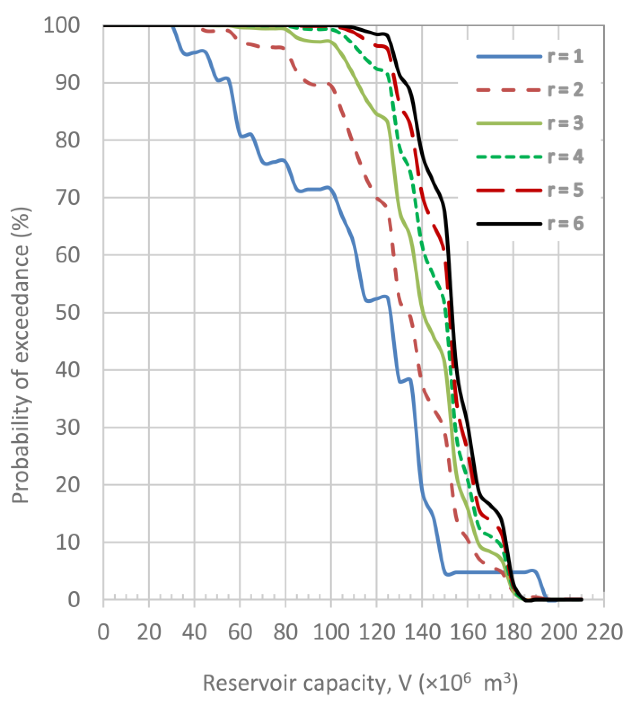
All the results, for each regulation period, are shown in Figure 3, where the cumulative frequency of exceedance, interpreted as probability of exceedance for any given reservoir capacity, is plotted for regulation periods r = 1 to r = 6 years.
One can observe that the reservoir capacity increases with increasing regulation periods, up to a practically limiting value of 184.45 × 10⁶ m3. This limiting value has very small probabilities for regulation periods of 1 and 2 years and probabilities very close to zero for longer regulation periods. It can also be observed that the curves corresponding to r = 5 and r = 6 are practically the same; this leads to the conclusion that the reservoir capacity, as a function of the regulation period, will not increase for longer regulation periods.
A second approach for tackling the problem of inflow data generation (hereafter called the Second Method) was based on the generation of a random year consisting of random precipitation values for each month, corresponding to the available monthly values for the 21 hydrologic years. The procedure, for a regulation period of 1 year is as follows:
- Twelve random integer numbers, R(I) with I = 1.12, were generated with values ranging from 1 to 21, which are the available hydrologic years of record.
- For each value of R(I), the corresponding month and its inflow were selected through a FORTRAN Do loop of the form:DO I = 1.12I1 = 12 × (R(I) − 1) + IF(I1) = MONTH (I1)END DOwhere MONTH(I1) contains, sequentially, the 12 × 21 = 252 values of inflow (see Table A1) for 21 consecutive years. This procedure ensures that a random monthly inflow (for each specific month) of the random year will be selected.
- For the year thus generated, the required reservoir capacity was computed.
- The procedure was applied for the generation of 1,000,000 random hydrologic years and the computation of the corresponding required reservoir capacities. The sample represents the 13.6 × 10⁻⁹% of all possible cases, which are equal to 2112 = 7,355,827,511,386,641.
The extension of the method for a multiple-year regulation period, r, is accomplished in a similar manner except that the random numbers are generated for 12 × r months. The method was used for the computation of reservoir capacities with regulation periods of 2, 3, 4, 5, 6, 8, and 10 years. For each regulation period, 1,000,000 hydrologic years were generated except for the regulation period of 10 years, where 1,621,958 hydrologic years were generated. The maximum of all required values for the reservoir capacity is summarized in Table 6.
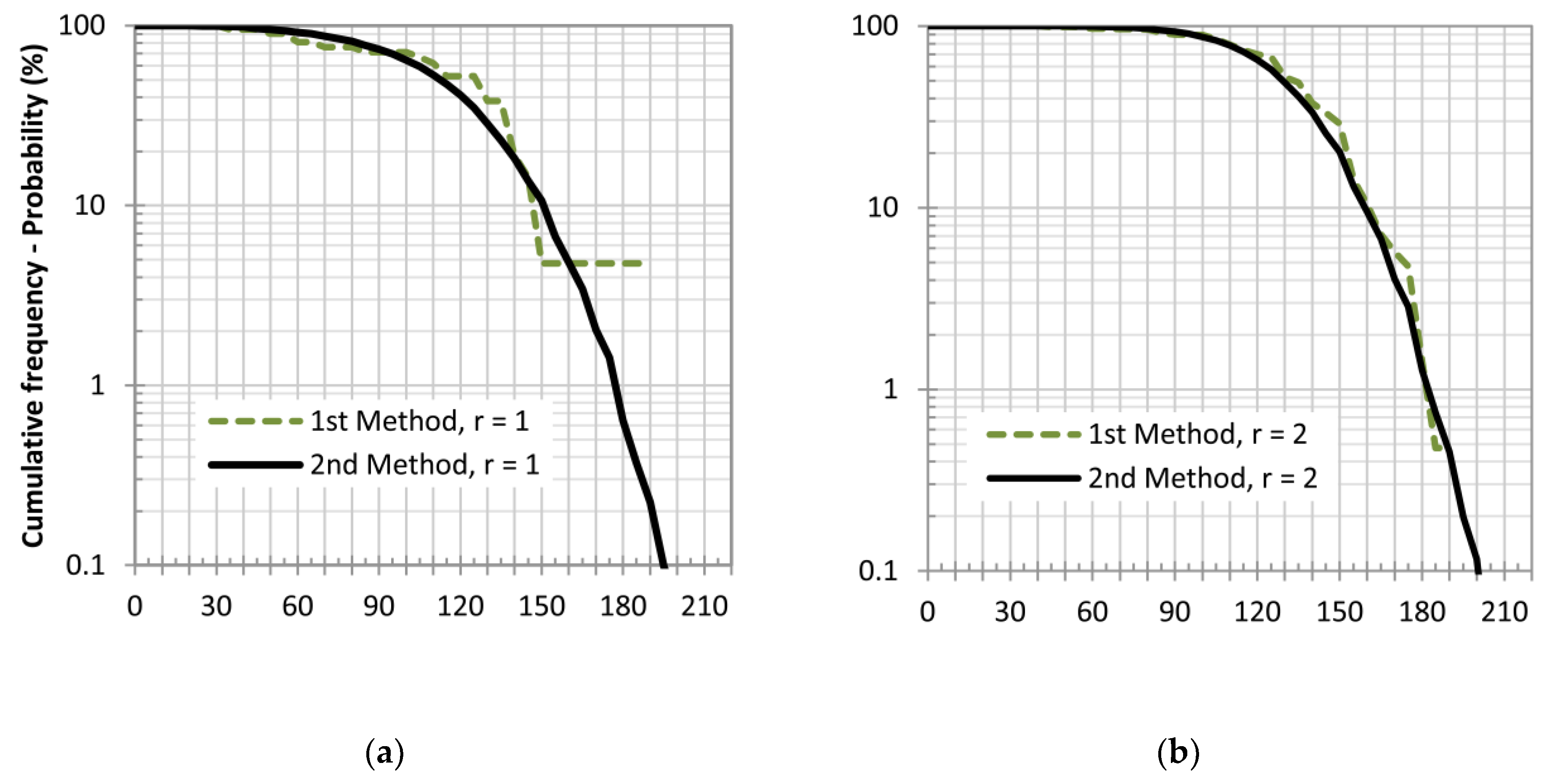
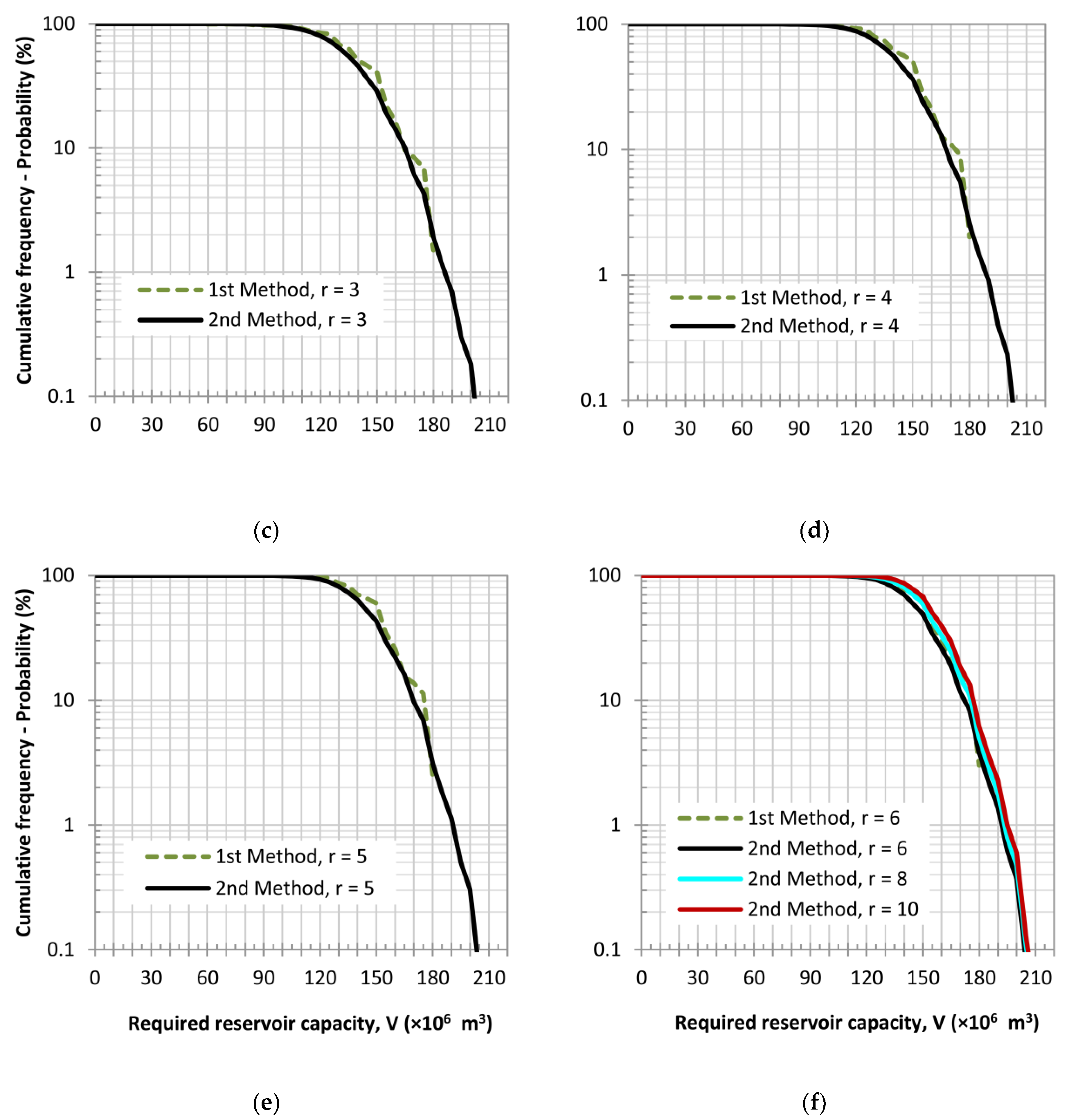
The results, from both methods and for each regulation period, are shown in Figure 4, where the cumulative frequency of exceedance, interpreted as probability of exceedance for any given reservoir capacity, is plotted for regulation periods r = 1 to r = 10 years. For instance, if the selected regulation period of the reservoir under consideration is three years, the required storage capacity would be 173 × 106 m3, 186 × 106 m3, and 203 × 106 m3 for 5%, 1%, and 0.1% probability of exceedance, respectively. The choice of the level of exceedance probability may be a matter of economic, social, and environmental factors; the lower the probability level the greater the reservoir storage capacity, hence the more expensive the project. These outcomes are necessary so that engineers may form alternative project budgets, which in turn are very significant to decision-makers for the final decision.
In summary, the First Method utilizes the combination of n = 21 years per k = 1, 2, 3, 4, 5, and 6 regulation years and subsequently performs all the permutations (k!) in each combination of k years, leading to a total of n!/(n − k)! cases. In the Second Method, hydrologic years were generated with inflow values for each month, randomly selected from the observed values for that month.
It is apparent from Figure 4 that both methods give practically the same results. This was expected, since the First Method essentially produces results, which can be viewed as a subset of the results of the Second Method. Furthermore, the Second Method has the advantage of allowing for the manipulation of a greater volume of data with practically the same ease for short or long regulation periods. It also requires much shorter computation times, that did not exceed 2 min for each case examined. Therefore, the present findings imply that the proposed Second Method is very robust and is suggested for use.
All computations were performed via codes written in FORTRAN 77 and the diagrams were prepared with EXCEL 2016.
4. Discussion and Conclusions
The focus of this study is on a general methodology for the determination of the required storage capacity of a reservoir, which is in the design phase. This entails two major components: (a) a method for the computation of reservoir active storage capacity, which is easier to interpret physically and implement computationally, and (b) an approach for the generation of a sequence of inflow data, for the desired period of reservoir regulation, from an available record of substantial length.
The computation of reservoir active storage capacity was performed with the aid of the concept of a zero-height dam proposed for the first time in the present work. The method is in the spirit of the methods initiated by Rippl; it is, however, easier to interpret physically and implement computationally.
Furthermore, the generation of appropriate inflow data assumes that a substantial record of monthly inflows is available along with predetermined monthly water demands. The treatment, however, of the inflow data for the generation of inflow sequences for any desired regulation period is quite different from other available methods and allows for the selection of the reservoir capacity for the desired level of probability of exceedance.
Although the two proposed methods give practically the same results, the Second Method is superior in terms of ease with which inflow sequences are generated. Also, due to the large size of the random sample that can be generated, the exceedance probability curves are very smooth and allow for the easy selection of the reservoir capacity with any level of desired probability of exceedance.
Finally, based on available monthly inflow and demand data, the present methodology provides a robust way to select reservoir capacity as a function of the reservoir regulation period and the exceedance probability. Thus, engineers can provide alternative project budgets useful for stakeholders and decision-makers.
Author Contributions
Conceptualization, P.C.Y. and A.C.D.; Methodology, P.C.Y.; Software, P.C.Y.; Validation, P.C.Y. and A.C.D.; Formal Analysis, P.C.Y.; Investigation, P.C.Y. and A.C.D.; Resources, P.C.Y.; Data Curation, P.C.Y.; Writing—Original Draft Preparation, A.C.D.; Writing—Review and Editing, P.C.Y. and A.C.D.; Visualization, P.C.Y. and A.C.D.; Project Administration, P.C.Y. and A.C.D.; Funding Acquisition, P.C.Y. and A.C.D.
Funding
This research received no external funding and the APC was funded through the Environmental and Hydraulic Engineering Laboratories.
Acknowledgments
The grant of 40% discount off the APC is acknowledged, in addition to the IOAP (https://www.mdpi.com/about/ioap) membership discount (10% for the University of Patras). Portion of this work was initiated while the authors were serving as adjunct faculty of the MSc Program “Engineering Project Management” at the Hellenic Open University.
Conflicts of Interest
The authors declare no conflict of interest.
Appendix A

Table A1.
Monthly and yearly precipitation heights (mm).
| No. | Hydrologic Year | Sep. | Oct. | Nov. | Dec. | Jan. | Feb. | Mar. | Apr. | May | Jun. | Jul. | Aug. | Year |
|---|---|---|---|---|---|---|---|---|---|---|---|---|---|---|
| 1 | 1974–1975 | 101.20 | 137.65 | 148.67 | 101.56 | 94.43 | 56.11 | 99.26 | 29.60 | 211.05 | 30.76 | 17.14 | 19.52 | 1046.96 |
| 2 | 1975–1976 | 0.00 | 49.12 | 222.86 | 262.69 | 133.90 | 134.41 | 27.73 | 150.33 | 38.18 | 29.46 | 59.35 | 0.00 | 1108.04 |
| 3 | 1976–1977 | 13.47 | 137.51 | 285.60 | 201.90 | 103.80 | 90.33 | 13.25 | 20.02 | 8.86 | 0.00 | 18.22 | 3.82 | 896.77 |
| 4 | 1977–1978 | 64.25 | 0.00 | 264.85 | 142.84 | 189.65 | 197.15 | 115.39 | 139.31 | 50.78 | 24.42 | 0.00 | 0.00 | 1188.64 |
| 5 | 1978–1979 | 72.32 | 100.91 | 217.60 | 143.34 | 238.42 | 92.56 | 66.27 | 154.43 | 90.04 | 14.77 | 9.51 | 46.75 | 1246.91 |
| 6 | 1979–1980 | 0.00 | 225.09 | 305.98 | 194.99 | 164.66 | 91.12 | 74.84 | 128.00 | 144.71 | 41.92 | 0.00 | 0.00 | 1371.31 |
| 7 | 1980–1981 | 20.82 | 191.89 | 151.41 | 231.72 | 178.35 | 146.29 | 39.18 | 87.80 | 49.70 | 26.58 | 35.73 | 19.16 | 1178.63 |
| 8 | 1981–1982 | 27.52 | 65.69 | 196.21 | 297.20 | 15.13 | 82.19 | 120.58 | 165.16 | 56.11 | 10.80 | 0.00 | 2.16 | 1038.74 |
| 9 | 1982–1983 | 51.86 | 154.14 | 222.57 | 294.10 | 46.53 | 103.58 | 56.18 | 18.01 | 0.00 | 46.10 | 96.52 | 33.13 | 1122.73 |
| 10 | 1983–1984 | 19.45 | 36.02 | 213.21 | 241.30 | 206.01 | 193.04 | 102.79 | 204.57 | 0.00 | 0.00 | 0.00 | 11.16 | 1227.54 |
| 11 | 1984–1985 | 10.08 | 0.00 | 83.27 | 118.85 | 206.01 | 157.75 | 87.16 | 59.06 | 0.00 | 0.00 | 0.00 | 0.00 | 722.17 |
| 12 | 1985–1986 | 0.00 | 34.57 | 176.47 | 156.31 | 179.35 | 113.09 | 113.09 | 18.73 | 51.86 | 7.92 | 0.00 | 0.00 | 851.39 |
| 13 | 1986–1987 | 0.00 | 169.99 | 27.37 | 203.84 | 155.58 | 166.39 | 127.49 | 56.90 | 10.08 | 0.00 | 0.00 | 38.90 | 956.56 |
| 14 | 1987–1988 | 54.02 | 99.40 | 239.14 | 133.98 | 107.32 | 146.22 | 107.32 | 33.13 | 38.18 | 0.00 | 0.00 | 0.00 | 958.72 |
| 15 | 1988–1989 | 11.52 | 94.36 | 198.80 | 105.88 | 0.00 | 24.49 | 28.81 | 69.87 | 42.50 | 0.00 | 0.00 | 0.00 | 576.24 |
| 16 | 1989–1990 | 0.00 | 121.73 | 90.04 | 110.93 | 0.00 | 57.98 | 0.00 | 36.02 | 27.37 | 0.00 | 0.00 | 13.69 | 457.75 |
| 17 | 1990–1991 | 38.18 | 83.55 | 65.55 | 307.57 | 41.78 | 60.00 | 71.53 | 87.52 | 67.71 | 11.52 | 24.49 | 6.41 | 865.80 |
| 18 | 1991–1992 | 0.00 | 39.90 | 46.46 | 33.49 | 7.49 | 2.88 | 29.10 | 68.79 | 10.88 | 7.20 | 30.61 | 0.00 | 276.81 |
| 19 | 1992–1993 | 9.65 | 9.87 | 26.15 | 39.76 | 9.87 | 99.26 | 64.47 | 31.19 | 72.25 | 18.08 | 0.00 | 0.00 | 380.53 |
| 20 | 1993–1994 | 2.59 | 14.19 | 159.98 | 121.01 | 100.55 | 142.40 | 32.63 | 66.77 | 49.05 | 0.00 | 29.17 | 15.49 | 733.84 |
| 21 | 1994–1995 | 0.00 | 54.02 | 131.09 | 130.01 | 164.95 | 72.03 | 108.41 | 12.61 | 24.85 | 0.00 | 7.92 | 7.92 | 713.82 |
Table A2.
Calculation of the required storage capacity, V (m3), for hydrologic year 1991–1992, with the lowest yearly inflow of 276.811 × 10⁶ m3.
Table A2.
Calculation of the required storage capacity, V (m3), for hydrologic year 1991–1992, with the lowest yearly inflow of 276.811 × 10⁶ m3.
| No. | Month | Inflow (×106) | Demand (×106) | Volume Deficit (−)/Surplus (+) | Cumulative Volume Deficit, V (×106) |
|---|---|---|---|---|---|
| 0 | 0.000 | ||||
| 1 | S | 0.000 | 25.099 | −25.099 | −25.099 |
| 2 | O | 39.905 | 25.099 | 14.806 | −10.293 |
| 3 | N | 46.459 | 10.099 | 36.360 | 0.000 |
| 4 | D | 33.494 | 10.099 | 23.395 | 0.000 |
| 5 | J | 7.491 | 10.099 | −2.608 | −2.608 |
| 6 | F | 2.881 | 10.099 | −7.218 | -9.825 |
| 7 | M | 29.100 | 10.099 | 19.001 | 0.000 |
| 8 | A | 68.789 | 25.099 | 43.690 | 0.000 |
| 9 | M | 10.877 | 25.099 | −14.222 | −14.222 |
| 10 | J | 7.203 | 41.974 | −34.771 | −48.993 |
| 11 | J | 30.613 | 41.974 | −11.361 | −60.354 |
| 12 | A | 0.000 | 41.974 | −41.974 | −102.328 |
| 13 | S | 0.000 | 25.099 | −25.099 | −127.427 |
| 14 | O | 39.905 | 25.099 | 14.806 | −112.621 |
| 15 | N | 46.459 | 10.099 | 36.360 | −76.261 |
| 16 | D | 33.494 | 10.099 | 23.395 | −52.866 |
| 17 | J | 7.491 | 10.099 | −2.608 | −55.473 |
| 18 | F | 2.881 | 10.099 | −7.218 | −62.691 |
| 19 | M | 29.100 | 10.099 | 19.001 | −43.690 |
| 20 | A | 68.789 | 25.099 | 43.690 | 0.000 |
| 21 | M | 10.877 | 25.099 | −14.222 | −14.222 |
| 22 | J | 7.203 | 41.974 | −34.771 | −48.993 |
| 23 | J | 30.613 | 41.974 | −11.361 | −60.354 |
| 24 | A | 0.000 | 41.974 | −41.974 | −102.328 |
References
- Yang, H.; Haynes, M.; Winzenread, S.; Okada, K. The History of Dams. 1999. Available online: https://watershed.ucdavis.edu/shed/lund/dams/Dam_History_Page/History.htm (accessed on 2 August 2018).
- Gupta, A. The World’s Oldest Dams Still in Use. Water Technology. 2013. Available online: https://www.water-technology.net/features/feature-the-worlds-oldest-dams-still-in-use/ (accessed on 2 August 2018).
- FAO. 2017. Available online: http://www.fao.org/nr/water/aquastat/dams/index.stm (accessed on 2 August 2018).
- Lehner, B.; Liermann, C.R.; Revenga, C.; Vörösmarty, C.; Fekete, B.; Crouzet, P.; Döll, P.; Endejan, M.; Frenken, K.; Magome, J.; et al. High-resolution mapping of the world’s reservoirs and dams for sustainable river-flow management. Front. Ecol. Environ. 2011, 9, 494–502. [Google Scholar] [CrossRef]
- Rippl, W. Capacity of storage reservoirs for water supply. Minutes Proc. Inst. Civ. Eng. 1883, 71, 270–278. [Google Scholar]
- American Society of Civil Engineers (ASCE). Hydrology Handbook, 2nd ed.; ASCE: Reston, VA, USA, 1996. [Google Scholar]
- Bharali, B. Estimation of Reservoir Storage Capacity by using Residual Mass Curve. J. Civ. Eng. Environ. Technol. 2015, 2, 15–18. [Google Scholar]
- Clark, J.W.; Viessman, W., Jr.; Hammer, M.J. Water Supply and Pollution Control, 3rd ed.; Harper & Row Publishers: New York, NY, USA, 1977. [Google Scholar]
- Thomas, H.A.; Fiering, M.B. Mathematical Synthesis of Streamflow Sequences for the Analysis of River Basins by Simulations. In Design of Water Resource Systems; Harvard University Press: Cambridge, UK, 1962; pp. 459–493. [Google Scholar]
- Şen, Z. A mathematical model of monthly flow sequences. Hydrol. Sci. J. 1978, 23, 223–229. [Google Scholar] [CrossRef]
- Langousis, A.; Koutsoyiannis, D. A stochastic methodology for generation of seasonal time series reproducing overyear scaling behaviour. J. Hydrol. 2006, 322, 138–154. [Google Scholar] [CrossRef]
- Oliveira, B.; Maia, R. Stochastic Generation of Streamflow Time Series. J. Hydrol. Eng. 2018, 23, 04018043. [Google Scholar] [CrossRef]
Figure 1.
Temporal variation of net inflow and net cumulative volume.

Figure 2.
Correlations of reservoir capacity V to: (a) yearly inflow; (b) standard deviation of monthly mean inflows/monthly mean; (c) skewness of monthly mean inflows; (d) kurtosis of monthly mean inflows.
Figure 2.
Correlations of reservoir capacity V to: (a) yearly inflow; (b) standard deviation of monthly mean inflows/monthly mean; (c) skewness of monthly mean inflows; (d) kurtosis of monthly mean inflows.

Figure 3.
Probability of exceedance for any given reservoir capacity and for regulation periods from 1 to 6 years.
Figure 3.
Probability of exceedance for any given reservoir capacity and for regulation periods from 1 to 6 years.

Figure 4.
Probability of exceedance for any given reservoir capacity with both methods and for a regulation period of (a) 1 year; (b) 2 years; (c) 3 years; (d) 4 years; (e) 5 years; (f) 6, 8, and 10 years.
Figure 4.
Probability of exceedance for any given reservoir capacity with both methods and for a regulation period of (a) 1 year; (b) 2 years; (c) 3 years; (d) 4 years; (e) 5 years; (f) 6, 8, and 10 years.


Table 1.
Computation of storage capacity for VT > 0.
| Year | Inflow (m3/s) | Demand (m3/s) | Volume Deficit (−)/Surplus (+) 1 | Cumulative Volume Deficit |
|---|---|---|---|---|
| 0 | 0 | |||
| 1 | 90 | 120 | −30 | −30 |
| 2 | 200 | 120 | 80 | 0 |
| 3 | 90 | 120 | −30 | −30 |
| 1 | 90 | 120 | −30 | −60 2 |
| 2 | 200 | 120 | 80 | 0 |
| 3 | 90 | 120 | −30 | −30 |
1 Volumes have been divided by 12 months × 30 days/month × 24 h/day × 3600 s/h = 31.104 × 10⁶ s. 2 Required storage: 60 × 31.104 × 106 = 1.866 × 10⁹ m3.
Table 2.
Computation of storage capacity for VT = 0.
| Year | Inflow (m3/s) | Demand (m3/s) | Volume Deficit (−)/Surplus (+) 1 | Cumulative Volume Deficit |
|---|---|---|---|---|
| 0 | 0 | |||
| 1 | 90 | 120 | −30 | −30 |
| 2 | 200 | 120 | 80 | 0 |
| 3 | 70 | 120 | −50 | −50 |
| 1 | 90 | 120 | −30 | −80 2 |
| 2 | 200 | 120 | 80 | 0 |
| 3 | 70 | 120 | −50 | −50 |
1 Volumes have been divided by 12 months × 30 days/month × 24 h/day × 3600 s/h = 31.104 × 10⁶ s. 2 Required storage: 80 × 31.104 × 106 = 2.488 × 10⁹ m3.
Table 3.
Computation of storage capacity for VT < 0.
| Year | Inflow (m3/s) | Demand (m3/s) | Volume Deficit (−)/Surplus (+) 1 | Cumulative Volume Deficit |
|---|---|---|---|---|
| 0 | 0 | |||
| 1 | 90 | 120 | −30 | −30 |
| 2 | 200 | 120 | 80 | 0 |
| 3 | 50 | 120 | −70 | −70 |
| 1 | 90 | 120 | −30 | −100 2 |
| 2 | 200 | 120 | 80 | −20 |
| 3 | 50 | 120 | −70 | −90 |
| 1 | 90 | 120 | −30 | −120 |
| 2 | 200 | 120 | 80 | −40 |
| 3 | 50 | 120 | −70 | −110 |
1 Volumes have been divided by 12 months × 30 days/month × 24 h/day × 3600 s/h = 31.104 ×10⁶ s. 2 Required storage: 100 × 31.104 × 106 = 3.11 × 10⁹ m3.
Table 4.
Monthly water demands (106 × m3/month).
| Month | Irrigation | Water Supply | Hydro-Power | Total |
|---|---|---|---|---|
| September | 15 | 1.875 | 8.224 | 25.099 |
| October | 15 | 1.875 | 8.224 | 25.099 |
| November | 0 | 1.875 | 8.224 | 10.099 |
| December | 0 | 1.875 | 8.224 | 10.099 |
| January | 0 | 1.875 | 8.224 | 10.099 |
| February | 0 | 1.875 | 8.224 | 10.099 |
| March | 0 | 1.875 | 8.224 | 10.099 |
| April | 15 | 1.875 | 8.224 | 25.099 |
| May | 15 | 1.875 | 8.224 | 25.099 |
| June | 30 | 3.75 | 8.224 | 41.974 |
| July | 30 | 3.75 | 8.224 | 41.974 |
| August | 30 | 3.75 | 8.224 | 41.974 |
Table 5.
Summary of results from the First Method.
| Years, r, of Regulation Period | Number of Combinations of 21 Years Per r Years | Total Number of Permutations | Maximum Reservoir Storage Capacity from All Computed Required Values (×106 m3) | Sequence of Years 1 for Each Regulation Period Corresponding to Maximum Reservoir Storage Capacity |
|---|---|---|---|---|
| 1 | 21 | 21 | 191.14 | 11 |
| 2 | 210 | 420 | 191.15 | 11–18 or 18–11 |
| 3 | 1330 | 7980 | 184.45 | 11–18–20 or 20–12–11 |
| 4 | 5985 | 143,640 | 184.45 | 1–11–18–20 or 20–12–11–18 |
| 5 | 20,349 | 2,441,880 | 184.45 | 1–2–11–18–20 or 20–2–1–11–18 |
| 6 | 54,264 | 39,070,080 | 184.45 | 1–2–3–11–18–20 and 3–4–5–11–18–20 or 20–3–2–1–11–18 and 20–5–4–3–11–18 |
1 Each number in this column corresponds to the enumeration of years, given in Table A1 of Appendix A.
Table 6.
Summary of results from the Second Method.
| Years, r of Regulation Period | Maximum Reservoir Capacity from All Computed Required Values (×106 m3) | Enumeration of Month Where Reservoir Capacity Becomes Zero | Size of Random Sample |
|---|---|---|---|
| 1 | 277.87 | 24 | 1,000,000 |
| 2 | 233.71 | 14 | 1,000,000 |
| 3 | 244.01 | 26 | 1,000,000 |
| 4 | 253.38 | 61 | 1,000,000 |
| 5 | 271.74 | 36 | 1,000,000 |
| 6 | 278.88 | 73 | 1,000,000 |
| 8 | 278.22 | 74 | 1,000,000 |
| 10 | 301.34 | 50 | 1,621,958 |
© 2018 by the authors. Licensee MDPI, Basel, Switzerland. This article is an open access article distributed under the terms and conditions of the Creative Commons Attribution (CC BY) license (http://creativecommons.org/licenses/by/4.0/).
Share and Cite
MDPI and ACS Style
Yannopoulos, P.C.; Demetracopoulos, A.C. A Novel Methodology for Multiple-Year Regulation of Reservoir Active Storage Capacity. Water 2018, 10, 1254. https://doi.org/10.3390/w10091254
AMA Style
Yannopoulos PC, Demetracopoulos AC. A Novel Methodology for Multiple-Year Regulation of Reservoir Active Storage Capacity. Water. 2018; 10(9):1254. https://doi.org/10.3390/w10091254
Chicago/Turabian StyleYannopoulos, Panayotis C., and Alexander C. Demetracopoulos. 2018. "A Novel Methodology for Multiple-Year Regulation of Reservoir Active Storage Capacity" Water 10, no. 9: 1254. https://doi.org/10.3390/w10091254
Note that from the first issue of 2016, this journal uses article numbers instead of page numbers. See further details here.