An Improved Grid-Xinanjiang Model and Its Application in the Jinshajiang Basin, China

Abstract

A modified form of the distributed Grid-Xinanjiang model (GXAJ) characterizing the infiltration excess and saturation excess runoff mechanisms coupled to a two-source potential evapotranspiration model (TSPE) was proposed to simulate the hydrological process and study the spatiotemporal pattern of the precipitation, evapotranspiration, and soil moisture in the Jinshajiang River basin. In the flow routing module, the flow is routed by the physically nonlinear Muskingum–Cunge method. The TSPE model can calculate the spatiotemporal variation of the potential canopy transpiration (CT), interception evaporation (IE), and potential soil evaporation (SE). Subsequently, the calculated potential evapotranspiration (PE) is coupled to the GXAJ model to calculate the water budget in each grid. An a priori parameter estimation was developed to obtain the spatially varied parameters from geographical data, including digital elevation model (DEM) data, soil data, vegetation data, and routing data. Hydrometeorological data were interpolated to 4750 grids with cell sizes of 10 km × 10 km by the Thiessen Polygon method. The DEM data was used to extract the flow direction, river length, hillslope, and channel slopes and to adjust the altitude-related meteorological variables. The reprocessed Moderate Resolution Imaging Spectroradiometer (MODIS) leaf area index (LAI) from the Beijing Normal University (BNU) dataset, which has a spatial resolution of 1 km × 1 km, was used to obtain the spatiotemporal variation in the LAI. The developed GXAJ model was applied to three sub-basins in the Jinshajiang River basin and was compared to the traditional GXAJ model. The developed GXAJ model satisfactorily reproduced the streamflow at each catchment outlet and matched the peak discharges better than the traditional GXAJ model for both the dry and wet seasons. The uneven distribution of the simulated mean annual evapotranspiration in the whole watershed was closely related to the vegetation types, ranging from 189.81 to 585.45 mm. Forest and woodland, shrubland, grassland, and cropland were shown to have mean annual evapotranspiration values of 485.6, 289.4, 275.9, and 392.3 mm, respectively. The ratios of the annual evapotranspiration to precipitation (E/P) of the forest, woodland, shrubland, grassland, and cropland were 54, 83, 53, and 48%, respectively.

1. Introduction

Hydrologists have developed various hydrological models for water and environment resource management over the past several decades. Traditionally, all of these hydrological models were classified as physically-based models or conceptually lumped models depending on the degree of complexity and physical completeness of the formulation of the structure [1]. The Xinanjiang (XAJ) model is a commonly used conceptual hydrological model which has a robust capacity to simulating hydrological processes in humid and semi-humid regions [2,3,4,5,6]. The XAJ model has also been demonstrated to achieve better results in dry catchments than the other four conceptual hydrological models, namely the Pitman model, the Sacramento model, the Nedbor-Afstromnings model (NAM) model, and Soil Moisture Accounting and Routing (SMAR) model [3].

Although the XAJ model can be successfully applied to flood forecasting, the simplified representation of the spatial distribution of the geospatial data of the drainage area and the consideration of the whole watershed as being one unit have been questioned. Furthermore, it also lacks the ability to predict the runoff in ungauged catchments and to assess the effects of human activities and climate change. Yao et al. [7] developed a distributed GXAJ model which incorporates the benefits of the widely used XAJ model and integrates the features of a distributed physically-based model. The GXAJ model divides the whole watershed into numerous computational grid cells. In each grid, the processes of evapotranspiration and runoff generation can be computed based on the initial XAJ model. The outflow of each cell to the basin outlet is routed from grid to grid along DEM-based river drainage networks by the Muskingum method. Yao et al. [7] proved that the GXAJ model surpasses the initial conceptual model in reproducing the outflow process in basin outlets, especially in large catchments. Yao et al. [8] noted that the GXAJ model still has some disadvantages. The model does not fully utilize physically a priori parameters, which hinders its application to other catchments and ungauged basins. For this reason, Yao et al. [7] developed an a priori parameter-estimated Grid-Xinanjiang model (PPGXAJ) based on the original GXAJ model. The PPGXAJ model derives many physically reasonable parameters from geographically-based original data, such as topographic information, soil texture, and land use/land cover data. The PPGXAJ model was applied to the Tunxi watershed with five internal stations to assess its ability to simulate hydrologic processes. The results showed that the developed model can represent the spatial variability in the geography and climate of the research basin and achieves satisfactory results in simulating the streamflow of the basin outlet and interior gauging stations without any recalibration.

The original conceptual XAJ model and the modified GXAJ model have been used successfully in many wet regions of China. However, without considering the infiltration excess runoff (IER) generation, the model faces a huge obstacle for wider implementation in sub-humid and semi-arid regions. Hu et al. [1] introduced a modified XAJ model combined with an infiltration and saturation excess runoff mechanism (ISER), which considers the mechanisms of both saturation excess runoff (SER) and IER. This model explicitly characterizes the impacts of different soil and precipitation conditions on the runoff generation and considerably expands the model’s application to the simulation of the rainfall runoff process in arid and semi-arid areas.

Evapotranspiration is a significant part of the hydrological cycle and is mainly affected by the soil vegetation system and weather conditions. In the classic XAJ model, the actual evapotranspiration (AE) is calculated by PE multiplied by a certain coefficient, which is determined by the soil moisture conditions. The PE is a fraction of the pan evaporation observations. However, this empirical calculation of PE cannot reflect the influences of and variation in the vegetation cover and land use. Ren and Guo [9] and Wang et al. [10] pointed out that the evaporation value measured by the evaporating dish is not always consistent or even negatively correlated under different environments. Penman [11] proposed an evapotranspiration method that considers energy and water transport mechanisms. Monteith [12] introduced aerodynamic resistance and surface resistance to calculate the evapotranspiration rates of different types of vegetation. The formula is named Penman–Monteith [13] and is widely used in hydrometeorological models. To calculate soil evaporation, Choudhury and Monteith [14] proposed the Choudhury–Monteith two-source evapotranspiration model (TSPE), which is better than the Penman–Monteith formula and is consistent with measured values. Yuan et al. [15] developed a hybrid form of the distributed model by integrating a physically based TSPE model with the GXAJ model. The TSPE model explicitly represents the spatiotemporal heterogeneity of PE, including potential CT, potential SE, and IE. The PE was then directly used to drive the Xinanjiang model to perform the streamflow simulation.

Although the XAJ model has experienced a variety of modifications, and each of the modified XAJ model has its advantages, as yet, there is no model that is comprehensive enough. There is currently no comprehensive model to integrate the advantages of each model. In addition, the above models all use the Horton infiltration formula to calculate the soil infiltration rate, but this formula mainly simulates the infiltration process of single field rainfall runoff, which cannot be applied to continuous rainfall runoff simulations. This paper uses the infiltration formula of Holtan [16], which obtains the infiltration rate according to the difference between the water storage capacity of the basin and the soil water content. The infiltration rate is independent of time and is only related to soil water content. Moreover, the Muskingum routing method or ‘lag and route’ technique adopted in the above GXAJ models cannot explicitly evaluate the impact of the depth of flow and surface roughness on the streamflow. Getirana et al. [17] coupled the nonlinear Muskingum–Cunge (NMC) routing method to a land surface model. This routing method is a physically-based method and has been demonstrated to be a robust solution.

In our research, an integrated form of the XAJ model is presented, which makes use of the strengths of the above-mentioned modified methods. The characteristics of the integrated model are as follows: (1) the development of a physically-based GXAJ model; (2) the ability to derive a priori parameters from geographically-based information; (3) surface runoff (SR) generation that dynamically considers the IER and SER mechanisms; (4) the utilization of a physically-based TSPE model to calculate the PE of each grid cell and (5) the calculation of flow routing using the NMC method. The proposed method is applied to the simulation of daily runoff in three subcatchments in the Jinshajiang River basin in China to evaluate its capability to simulate the runoff generation and water budget and to assess the spatiotemporal patterns of the precipitation, evapotranspiration, and soil moisture in the Jinshajiang River basin.

2. Improved GXAJ Model Formulation

2.1. Two-Source Potential Evapotranspiration (TSPE) Model

PE is the theoretical maximum amount of water that can dissipate into the air from a land surface with continuous coverage and sufficient water [18,19]. The TSPE model was developed by Yuan et al. [15] as an improved form of a two-source evaporation model [20] to calculate the potential CT ($E_{pc}$), potential SE ($E_{ps}$), and IE ($E_i$), which Mo et al. [20] characterized by calculating the energy balance and evapotranspiration of the sparse canopy. The three components can be calculated as follows:

$$E_{pc}=\frac{\Delta R_{nc}+\frac{\rho C_p{D}_0}{{\mathrm{r}}_{ac}}}{\lambda \left[\Delta +\gamma (1+\frac{r_{cp}}{r_{ac}})\right]}(1-W_{fr})$$

(1)

$$E_i=\frac{\Delta R_{nc}+\frac{\rho C_p{D}_0}{r_{ac}}}{\lambda (\Delta +\gamma )}{W}_{fr}$$

(2)

$$E_{ps}=\frac{\Delta (R_{ns}-G)+\frac{\rho C_p{D}_0}{{\mathrm{r}}_{as}}}{\lambda \left[\Delta +\gamma (1+\frac{r_{sp}}{r_{as}})\right]}$$

(3)

where $R_{nc}$ and $R_{n\mathrm{s}}$ are the net amounts of radiation absorbed by the canopy and soil (W m⁻²), respectively; G is the soil heat flux (W m⁻²); $\lambda$ is the latent of vaporization (MJ kg⁻¹); $\rho$ is the air density (kg m⁻³); $C_{\mathrm{p}}$ is the air specific heat at constant pressure (KJ kg⁻¹ °C⁻¹); $\gamma$ is the psychrometric constant (kPa °C⁻¹); $\Delta$ is the slope of the saturation vapor pressure–temperature relationship (kPa °C⁻¹); $W_{fr}$ is the wetted fraction of the canopy; $r_{ac}$ and $r_{as}$ are the bulk boundary layer resistance of the canopy and the aerodynamic resistance between the soil surface and the canopy air space (sm⁻¹), respectively; $r_{cp}$ and $r_{sp}$ are the bulk stomatal resistance of the canopy and the soil surface resistance with the soil moisture at field capacity (sm⁻¹), respectively; and $D_0$ is the saturation vapor pressure deficit at the source height (kPa).

2.2. Infiltration and Saturation Excess Runoff Model (ISER)

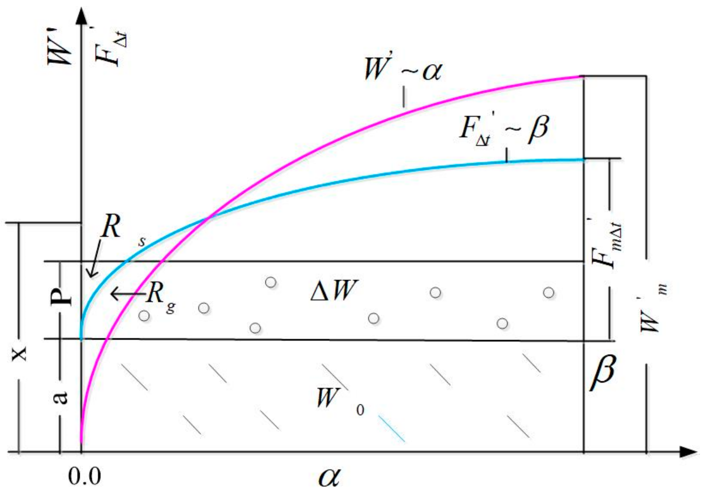
During most rainfall runoff events, excess infiltration and excess storage often occur alternatively. Infiltration runoff occurs when the rate of the intensity of the rainfall exceeds the infiltration rate, while saturation runoff occurs if the soil water content goes beyond its field capacity [1,19,21]. Figure 1 shows the schematic diagram of the runoff method. The curve $W^{\prime }~\alpha$ represents the special heterogeneity of the tension water capacity (TWC), which is determined by the specific watershed and is unalterable. The curve $F_{\Delta t}{}^{\prime }~\beta$ represents the spatial distribution of the soil infiltration capacity (SIC). It is based on the soil water content and varies during different time intervals. With changes in the precipitation and soil moisture content, the $F_{\Delta t}{}^{\prime }~\beta$ curve changes, which makes the R_s (SR) and R_g (groundwater runoff, GR) different. X is the distance from the intersection of curve $W^{\prime }~\alpha$ and curve $F_{\Delta t}{}^{\prime }~\beta$ to the origin. These two curves can be presented using the following equations:

$$\alpha =1-(1-\frac{W^{\prime }}{W_M{}^{\prime }}{)}^b$$

(4)

$$\beta =1-{(1-\frac{F_{\Delta t}{}^{\prime }}{F_m{{}_{\Delta t}}^{\prime }})}^B$$

(5)

where $W^{\prime }$($F_{\Delta t}{}^{\prime }$) and $W_m{}^{\prime }(F_{m\Delta t}{}^{\prime });$ are the TWC point (SIC point) and the maximum value of TWC (the maximum value of SIC), respectively; $b$(B) is an empirical exponential; $\alpha$ represents the area fraction of the runoff in which precipitation exclusively generates runoff; and $\beta$ is the area fraction of SR in which the rate of the rainfall intensity is greater than the infiltration rate. The spatial average point infiltration function can be derived using the Holtan equation [16]:

$$f_t=f_c+a{(S-F)}^n$$

(6)

where $a$ is the average basal area of the plant stems expressed as a fraction of the total area (0.25 < a < 0.8); S is the potential storage of soil moisture (mm); F is the total amount of infiltration (mm); n is an exponent (1.4); $f_c$ is the steady-state infiltration rate (mm/h); and $f_t$ is the point infiltration rate (mm/h).

S is equal to $W_M$(mean TWC), which is described by the following equation:

$$W_M=\frac{W^{\prime }{}_M}{1+b}$$

(7)

This equation is time-independent and is related to the soil moisture content, which makes it suitable for a consecutive simulation.

2.3. Nonlinear Muskingum–Cunge Routing Method

The parameters K and X of the NMC method are physically based and can be derived from in situ and satellite data, which distinguishes this method from the Muskingum method. The parameters K and X can be expressed as follows:

$$K=\frac{\Delta x^{\prime }}{c_0}$$

(8)

$$X=\frac{1}{2}-\frac{q_0}{w{S}_0{c}_0\Delta x^{\prime }}$$

(9)

$$c_0=\frac{5}{3}\frac{q_o^{0.4}{S}_o^{0.3}}{n^{0.6}{w}^{0.4}}$$

(10)

$$w=12A^{0.17}$$

(11)

$$q_o^t=\frac{Q_i^{t-1}+Q_i^t+Q_o^{t-1}}{3}$$

(12)

where $c_0$ (m s⁻¹) is the kinematic wave celerity; $q_0$ (m³ s⁻¹) is the reference discharge; $S_0$ is the river bed slope, which can be retrieved from DEM data; w (m) and $\Delta x^{\prime }$ are the width and length of a river reach; and N stands for Manning’s n and can be estimated with the help of relevant literature [17]. For each cell, $Q_o^{t-1}(m^3\Delta t^{-1})$ represents the discharge at time t − 1. $Q_i^{t-1}({\mathrm{m}}^3\Delta t^{-1})$ and $Q_i^t({\mathrm{m}}^3\Delta t^{-1})$ are the inflows at times t − 1 and t.

2.4. Schematic Diagram of the Integration of the ANNs with Conceptual Models

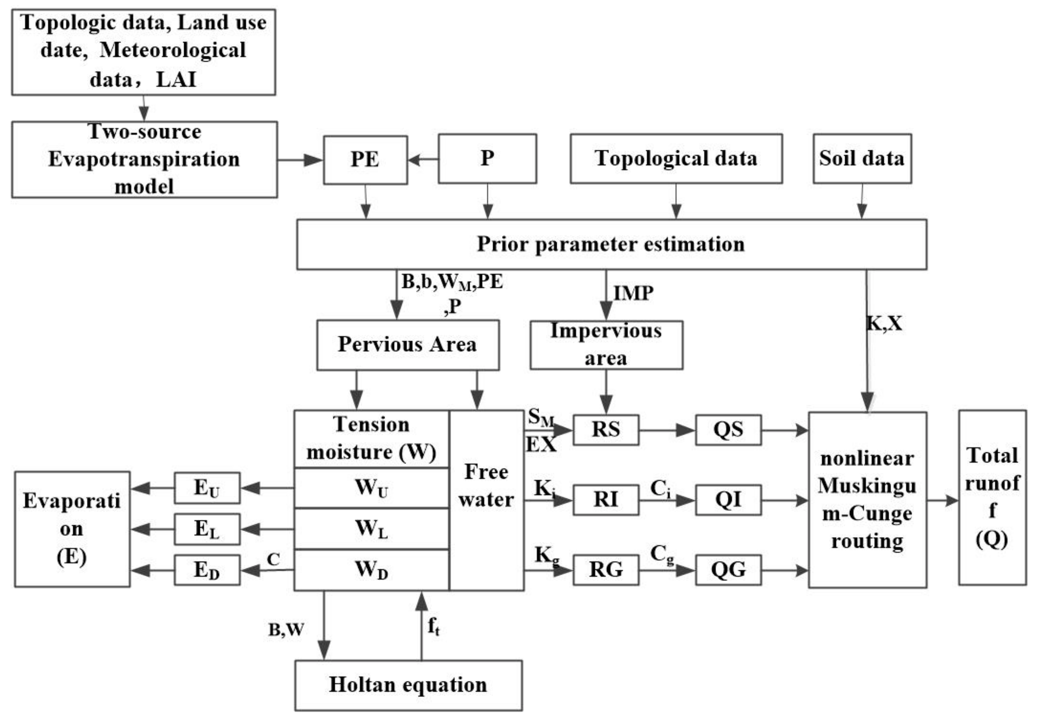
The developed GXAJ model was incorporates TSPE, GXAJ, ISER, and NMC for daily runoff simulations. A schematic chart of the hybrid model is illustrated in Figure 2. As shown in the Figure 2, the hybrid model contains five parts: PE, AE, runoff generation, runoff separation, and river routing. The inputs to the model are topologic data, land use data, meteorological data, the leaf area index (LAI), and soil data. The output is the streamflow at the basin outlet. The TSPE model is firstly used to calculate the PE. The PE and precipitation are then input to the ISER model to obtain the total runoff. The total runoff is then reallocated to SR, interflow, and GR based on a free water capacity (FWC) distribution curve. The AE is calculated by PE and the evapotranspiration coefficient of the deeper layer, with consideration of the soil storage deficit. The input SR, interflow, and GR are then adjusted by a recession constant into the nonlinear Muskingum–Cunge routing model.

3. A Brief Description of the Study Area

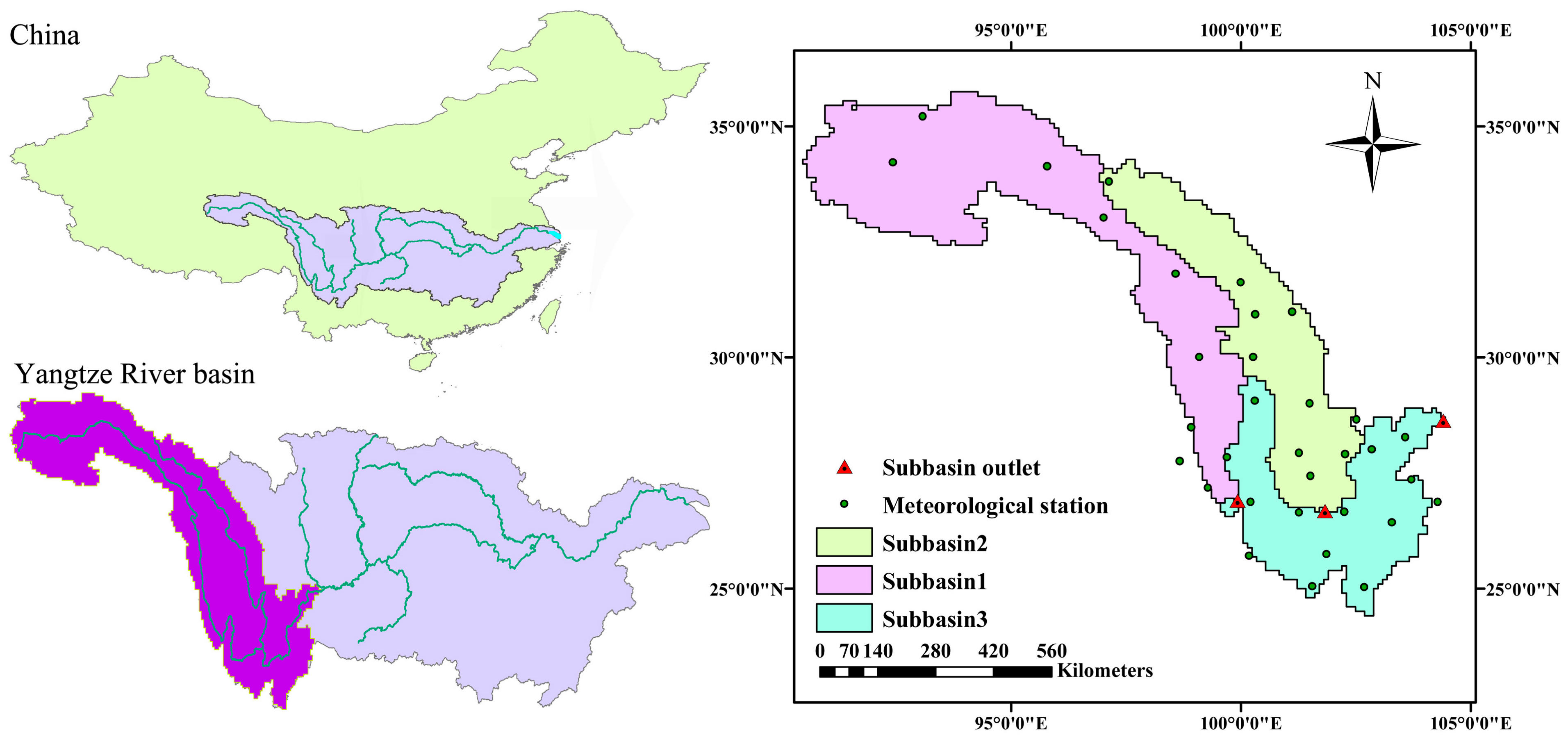
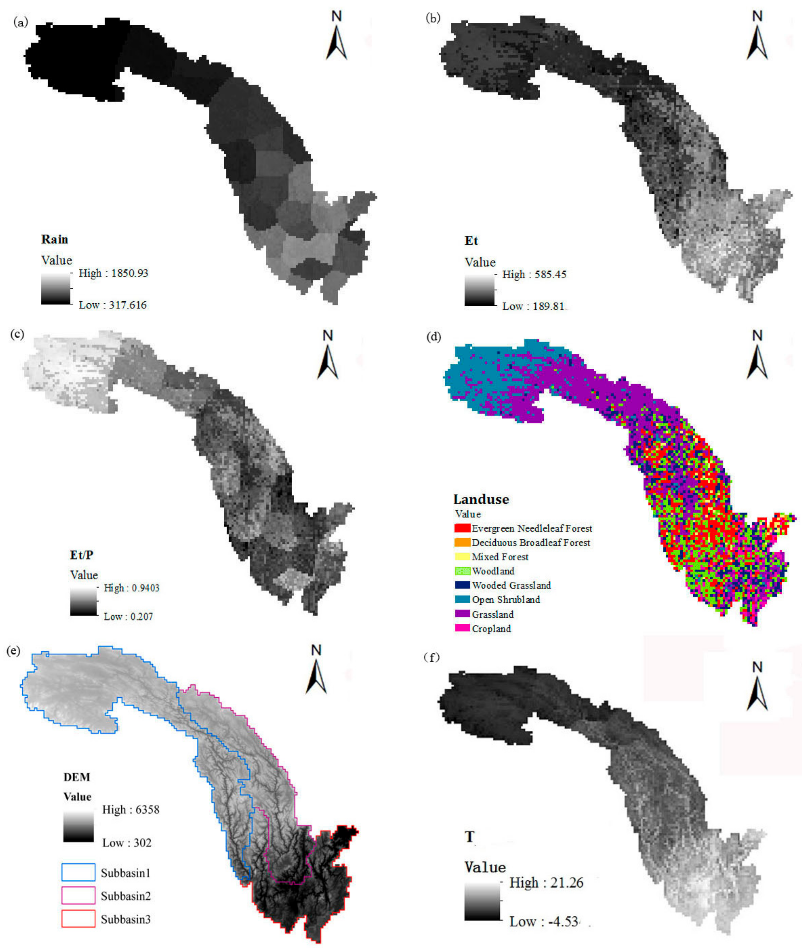
The Jinshajiang River basin is the source of the Yangtze River Basin and is located in southwest China. The Jinshajiang River flows through the Tibet, Qinghai, Sichuan, and Yunnan provinces. The basin is characterized by broad climate zones, varying from humid to semi-arid environments, and has a large drainage area of 458.8 × 10³ km². The mean annual temperature ranges from −4.5 °C to 16.4 °C. The total annual rainfall varies from 321 to 1662 mm. Approximately 85% of the annual total rainfall occurs during the monsoon months, from May to September, with strong spatial and temporal variation. Based on the river network characteristics, the Yangtze River Basin can be delineated into three sub-basins, as illustrated in Figure 3. Sub-basin 1, located in the Southeastern part of the Tibet Plateau, is upstream of the Jinshajiang River.

Table 1. The annual characteristics of three sub-basins of the Jinshajiang River basin [23].

Watershed	Area (km2)	Evaporation (mm)	PE (mm)	Temperature (°C)	Runoff (mm)	Runoff Coeff	Climate Zone
Sub-basin 1	214,184	461.5	1351.54	0.44	201.90	0.44	Semi-arid, semi-humid
Sub-basin 2	136,000	753.16	1264.57	7.43	446.16	0.59	Semi-humid
Sub-basin 3	108,616	909.76	1267.21	13.52	479.53	0.53	Humid

and alpine valleys make the region a transition zone from shrubland and grassland to forest. With a high topographic relief, Sub-basin 2, the largest tributary to the Jinshajiang River, has rich water resources. The main vegetation types of this sub-basin are forest, grassland, and cropland. Sub-basin 3, located downstream, is the more populated area and has ample rainfall. This area is covered by forest, woodland, grassland, and cropland. The annual characteristics of the three sub-basins are listed in Table 1.

4. Materials and Methods

4.1. Topographical Land Cover Data

The 3 × 3 arcs of DEM were obtained from the shuttle radar topography mission (SRTM) website (http://www.cgiar-csi.org/data). The land cover data were obtained from the University of Maryland at a spatial resolution of 30 × 30 arcs, including 14 classifications. The main vegetation types of the Jinshajiang River basin are forest, woodland, grassland, shrubs, and crops.

4.2. Modis LAI

The LAI data were provided by the BNU MODIS LAI dataset (http://globalchange.bnu.edu.cn), which offers global LAI data from 2000 to 2009 in 8-day intervals at a 1-km spatial resolution. This dataset is based on the original Moderate Resolution Imaging Spectroradiometer (MODIS) LAI product (MOD15A2) (https://modis.gsfc.nasa.gov/), with reduced deviation caused by cloudiness, snow, and some other issues.

4.3. Meteorological Data

The daily data of 33 meteorological stations from 2001 to 2008, including mean, maximum, and minimum temperatures, air vapor pressure, wind velocity, daylight duration, and precipitation, were acquired from the China Meteorological Administration. The calibration period considered was 2001–2005 for the daily observed streamflow, and data from 2006 to 2008 were used to validate the model. All meteorological data were interpolated over the whole basin at a 10-km resolution using the Thiessen Polygon method. At the same time, some climate variables corresponding to DEM, such as temperature, air vapor pressure, wind velocity, and rainfall, were topographically corrected using the empirical equations proposed by Fu and Lu [24].

4.4. A Prior Parameter Estimation

The availability of physically derived parameter estimates can effectively improve our understanding of the spatial characteristic of the study area and reduce the cost of computation. The parameters W_U (TWC of upper layer), W_L (TWC of lower layer, EX (exponential parameter of C_g (recession constant of groundwater storage), and IMP (fraction of impervious area) have less influence on the model outputs, while K_i (outflow coefficient of free water storage, FES, to interflow), K_g (outflow coefficient of the free water storage (FWS) to groundwater), C (evaporation coefficient of deeper layer), C_i (Recession constant of interflow storage), b, S_M (FWC), and W_M are sensitive parameters [25,26,27,28]. The empirical relations were used to estimate W_U, W_L, and C_g, as follows: $W_U=0.167\times W_M$, $W_L=0.5\times W_M$ (Yao et al. 2012), and $C_g=Q_{t+1}/Q_t$ (outflow of dry season at times t + 1, t), EX, and IMP were set to 1.5, and 0.01, respectively [19]. WM and SM correspond to the soil texture and vegetation type and were estimated from the following equations:

$$W_m=({\theta }_{fc}-{\theta }_{wp})\times L_a$$

(13)

$$S_m=({\theta }_{\mathrm{s}}-{\theta }_{fc})\times L_h$$

(14)

$$L_h={\vartheta }_{lc}{L}_a$$

(15)

where ${\theta }_{\mathrm{s}}$ is the saturated moisture content; ${\theta }_{fc}$ is the field moisture capacity; ${\theta }_{wp}$ is the wilt point; $L_a$ is the thickness of the aeration zone; $L_h$ is the thickness of humus soil; and the ${\theta }_{\mathrm{s}}$, ${\theta }_{fc}$, and ${\theta }_{wp}$ of each type of soil were derived from Anderson et al. [29] and Yao et al. [7]. The parameter $T{I}_i$ is the topographic index of each grid (i) and is obtained from DEM. The parameter ${\vartheta }_{lc}$ is the adjustment coefficient and can be obtained by referring to Yao et al. [8]. The coefficients ${\xi }_a$ and ${\xi }_b$ can be estimated from the following equations:

$${\xi }_a\times T{I}_{\min }+{\xi }_b{=L}_{a\max }=\frac{W_{M\max }}{{\theta }_{fc,T{I}_{\min }}-{\theta }_{wp,T{I}_{\min }}}$$

(16)

$${\xi }_a\times T{I}_{\max }+{\xi }_b{=L}_{a\min }=\frac{W_{M\min }}{{\theta }_{fc,T{I}_{\max }}-{\theta }_{wp,T{I}_{\max }}}$$

(17)

Based on related literature [8,19], the areal mean of $W_M$ was set as 100 for the humid region and 150 for the semi-humid region. The parameters $W_{M\max }=(1+b)\times W_M$ and $W_{M\min }$ are set to zero. The parameters K_i and K_g control the outflow rate of the interflow and groundwater from FWS. They are estimated according to Koren et al. [30]. The optimum values of b, B, C, C_i, and a for different sub-basins are determined by an optimization algorithm (SCE-UA; Duan et al. [31,32]). The hybrid model was calibrated for the period of 2001–2005 and was validated for the period of 2006–2008. The description and acquisition methods of all model parameters are shown in

Table 2. The description and acquisition methods of all model parameters.

Module	Parameter	Description	Acquisition Method
Two-source potential evapotranspiration	rmin	minimum stamatal resistance(sm−1)	based on land data assimilation system (LDAS)
	ac	albedo	based on land data assimilation system (LDAS)
	h	height of vegetation(m)	based on land data assimilation system (LDAS)
	Wmax	maximum leaf width	based on land data assimilation system (LDAS)
	d0	monthly zero-plane displacement	based on land data assimilation system (LDAS)
	z0	monthly roughness length	based on land data assimilation system (LDAS)
	LAI	Leaf area index	from the BNU MODIS LAI dataset
Actual evaporation	Wum	tension water capacity (TWC) of upper layer (mm)	Based on WM
	Wlm	TWC of lower layer (mm)	Based on WM
	C	evapotranspiration coefficient of deeper layer	determined by optimization algorithm
Runoff generation	Wm	TWC (mm)	using θfc, θwp, and aeration zone thickness
	θs	saturated moisture content	from literature
	θfc	field capacity	from literature
	θwp	wilting point	from literature
	Sm	free water capacity (FWC; mm)	using θs, θfc, and humus layer thickness
	Ki	outflow coefficient of FWS to interflow	on the basis of soil properties
	Kg	outflow coefficient of FWS to groundwater	on the basis of soil properties
	Ci	recession coefficient of interflow water	determined by optimization algorithm
	Cg	recession coefficient of groundwater water	outflow of dry season at time t+1, t
Nonlinear Muskingum–Cunge routing method	n	Manning roughness coefficient	from literature
	q0	water discharge of reference(m3s−1)	using outflow and inflow of each grid
	S0	river bed slope	derived from the shuttle radar topography mission (SRTM) digital elevation model (DEM)
	w	width of a river reach (m)	derived from the drainage area
	Dx′	length of a river reach(m)	using total river length within each grid
Infiltration and saturation excess runoff	b	exponent of TWC capacity distribution curve	determined by optimization algorithm
	B	exponent of soil infiltration capacity distribution curve	determined by optimization algorithm
	a	average basal area of plant stems	determined by optimization algorithm

.

The results were evaluated by four statistical indices including the Nash and Sutcliffe efficiency coefficient (NSE) [33], the relative error (RE), the percentage error in peak flow rate (PEP) and the percentage error in wave volume (PEV) [34].

$$\mathrm{NSE}=(1-\frac{{\displaystyle \sum (Q_o-Q_s{)}^2}}{{\displaystyle \sum (Q_o-{\overline{Q}}_o{}^2}})\times 100$$

(18)

$$\mathrm{RE}=(\frac{{\displaystyle \sum _i{Q}_o}}{{\displaystyle \sum _i{Q}_i}}-1)\times 100$$

(19)

$$\mathrm{PEP}=(\frac{Q_{s,\max }}{Q_{o,\max }}-1)\times 100$$

(20)

$$\mathrm{PEV}=(1-\frac{V_s}{V_o})\times 100$$

(21)

where $Q_o$ is the measured runoff (m³/s); $Q_s$ is the simulated runoff (m³/s); ${\overline{Q}}_{\mathrm{o}}$ is the mean values of the measured runoff (m³/s); $Q_{s,\max }$ is the simulated peak discharge; $Q_{o,\max }$ is the observed peak discharge; $V_s$ is the simulated volume of hydrograph; and $V_o$ is the observed volume of hydrograph.

This paper used the generalized likelihood uncertainty estimation (GLUE) method to analyze the uncertainty of the model parameters [35]. The method randomly generates a large number of parameter sets sampled from proposed (prior) distributions and inputs them into the model. Based on the selected likelihood function, the likelihood function values between the simulated results and the observed results are calculated. Here, the parameter prior distribution adopts the most commonly used uniform distribution [34] and samples the parameters uniformly within the parameter value range. The Nash–Sutcliffe efficiency [33] is selected as the likelihood objective function. The average relative length (ARL) [36], average asymmetry degree (AAD) [37] and average deviation amplitude (ADA) [37] are used to quantify the model’s uncertainty.

$$\mathrm{ARIL}=\frac{1}{n}{\displaystyle {\sum }_{i=1}^n\frac{Limi{t}_{u,t}-Limi{t}_{l,t}}{Q_{o,t}}}$$

(22)

$$\mathrm{ADD}=\frac{1}{n}{\displaystyle {\sum }_{i=1}^n\left|\frac{Limi{t}_{u,t}-Q_{o,t}}{Limi{t}_{u,t}-Limi{t}_{l.t}}-0.5\right|}$$

(23)

$$\mathrm{ADA}=\frac{1}{n}{\displaystyle {\sum }_{i=1}^n\left|\frac{1}{2}(Limi{t}_{u,t}+Limi{t}_{l,t})-Q_{o,t}\right|}$$

(24)

where $Q_o$ is the measured runoff (m³/s), and $Limi{t}_{u,t}$ and $Limi{t}_{l,t}$ are the upper and lower boundary values of 95% confidence intervals respectively.

5. Results and Discussion

5.1. Evaluation of the Simulated Streamflow

Table 3. Performances of the three sub-basins in the modified GXAJ model, ISER + GRAJ model, and TSPE + GRAJ model (daily).

Parameter	Category	Calibration			Validation
		Sub-Basin 1	Sub-Basin 2	Sub-Basin 3	Sub-Basin 1	Sub-Basin 2	Sub-Basin 3
Modified GRAJ Model
NSE (%)	mean annual flow	95.39	88.97	94.80	94.81	88.35	95.63
	rainy season	91.26	83.54	92.19	91.58	85.03	93.86
	dry season	81.68	61.06	82.82	76.94	58.49	87.70
RE	mean annual flow	−2.60	−6.51	1.41	4.26	−6.88	1.20
	rainy season	−3.65	−5.97	1.11	3.46	−4.53	2.97
	dry season	4.95	−11.10	2.43	8.27	−12.77	−3.97
PEP	rainy season	−3.80	−9.80	−4.40	−4.80	−8.60	−3.40
PEV	rainy season	−6.50	−11.50	2.60	6.13	−8.65	5.35
ISER + GRAJ Model
NSE	mean annual flow	94.22	86.68	93.34	93.59	85.87	94.66
	rainy season	89.29	81.87	90.05	90.02	83.10	93.00
	dry season	80.34	62.18	80.95	74.34	56.67	85.37
RE	mean annual flow	−3.70	−6.88	−2.10	4.65	−6.30	-2.50
	rainy season	−4.50	−6.60	−1.82	4.12	−5.70	−2.90
	dry season	6.20	−12.00	−4.20	8.67	−11.90	3.50
PEP	rainy season	−4.60	−10.10	−5.10	−5.30	9.50	−4.10
PEV	rainy season	−7.10	−13.20	−4.30	7.32	−12.46	−5.12
TSPE + GRAJ Model
NSE	mean annual flow	92.33	81.90	91.16	92.59	76.98	90.66
	rainy season	87.17	80.44	89.15	87.66	80.30	92.32
	dry season	75.60	60.66	76.90	69.38	56.99	82.46
RE	mean annual flow	−8.03	−7.83	−2.01	−5.12	−8.94	−3.31
	rainy season	−7.90	−7.37	−2.53	−4.17	−7.24	−2.90
	dry season	−8.23	−12.00	5.62	−9.46	−15.30	−7.42
PEP	rainy season	−9.70	−12.40	−7.70	−9.20	−11.70	−6.20
PEV	rainy season	−14.50	−16.30	−7.05	−8.47	−14.87	−5.31

presents the performance of the three sub-basins using the modified GXAJ model, the ISER + GRAJ model, and the TSPE + GRAJ model. We evaluated three periods of flood discharge, including the mean annual flow, the dry season flow (January–April, November–December), and the rainy season flow (May–October). In addition, during the dry period, the flood peak was not significant, so PEV and PEP were calculated for the rainy season). Table 3 shows that these three methods achieved satisfactory simulations for the periods of mean annual flow and the rainy season, with NSE values larger than 0.8, and the modified GXAJ model and ISER + GRAJ model performed better than the TSPE + GRAJ model, especially in the semi-arid and semi-humid region (Sub-basin 1). The results of the modified GXAJ model and the ISER + GRAJ model are similar to each other, because, as Wang et al. [10] pointed out, the correlation between the measured results of evaporating dishes in the upper reaches of the Yangtze river and the actual evaporation values is positive. At the same time, the runoff volume in the basin is large, so the difference of evaporation has little influence on the runoff simulation results.

Compared to the performances of Sub-basin 1 and Sub-basin 3, Sub-basin 2 showed relatively worse results in each evaluation period. Water projects of all sizes have been established there during the last decade because of the abundant water resources, and the features of snow-fed alpine valleys make the hydrological process complex. Sub-basin 1 achieved good results in both calibration and validation periods, even though it is a transition zone from semi-arid to semi-humid. Sub-basin 1 is situated southeast of the Tibet Plateau, and it is characterized by bad weather, poor traffic, a vast and sparse population, and natural flow.

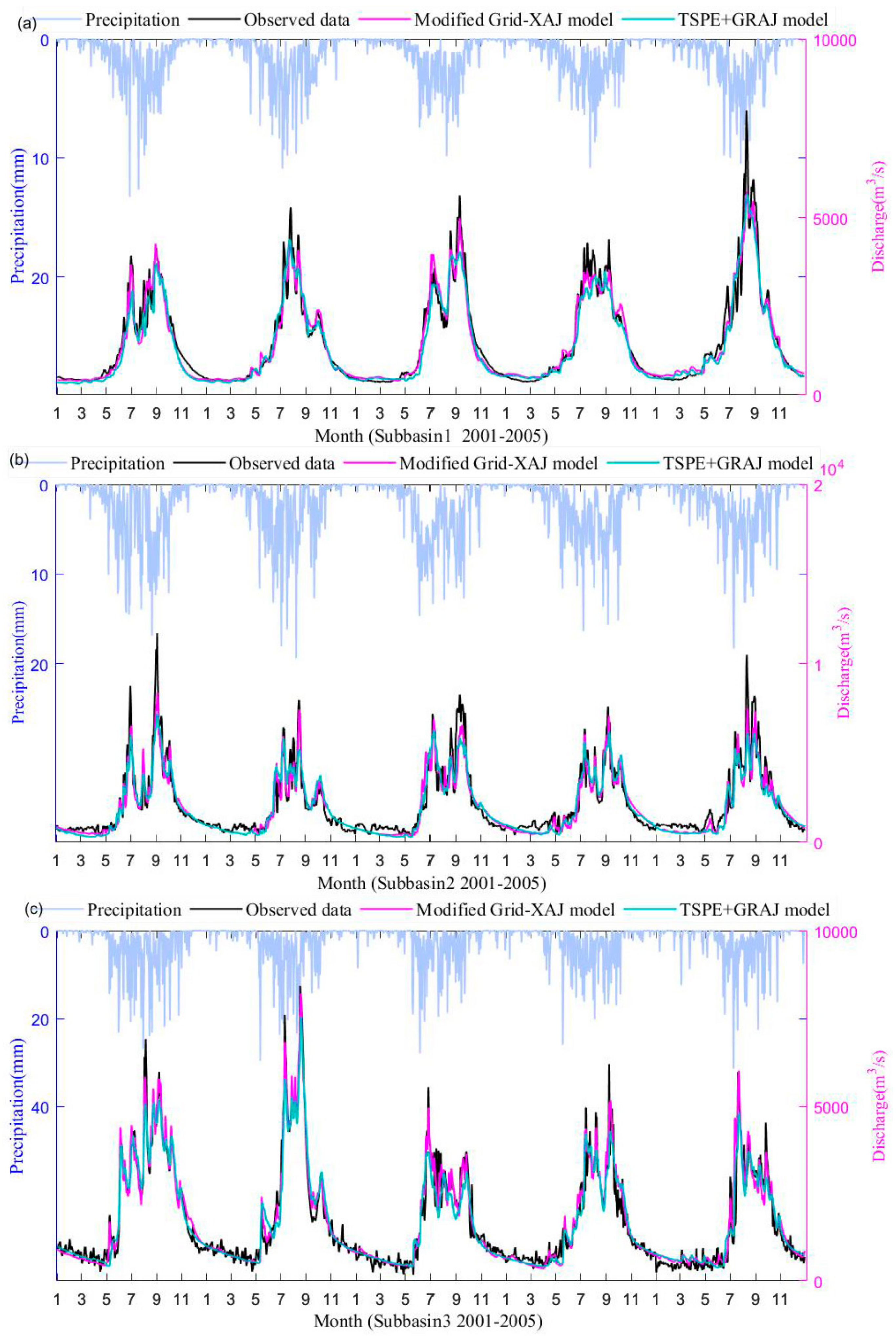
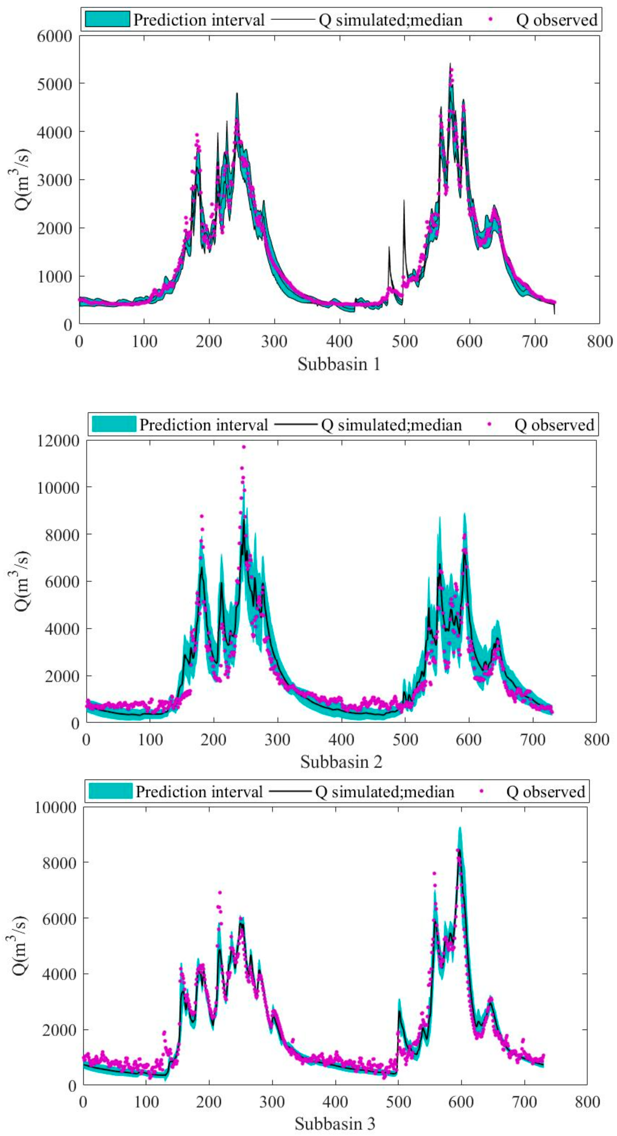
Since the values measured by the evaporating dish in the upper reaches of the Yangtze River were consistent with the actual evaporation trend, the results of the modified GXAJ model and ISER + GRAJ model were less different. We focused on comparing the results of the modified GXAJ model and the TSPE + GRAJ model. Figure 4a–c show the time series of the observed and estimated daily streamflow hydrographs from the modified GXAJ model and the TSPE + GRAJ model in the calibration period. Figure 4 shows that the simulated outflows of the two GXAJ models were consistent with the observed outflow series, while the modified GXAJ model performed better than the TSPE + GRAJ model in simulating the peak discharge of the runoff processes for both the rainy and dry seasons. In the rainy season, the rainfall intensity rate may be larger than the infiltration rate in some regions, and in the dry season, the infiltration rate of the water-starved soil may be smaller than the rainfall. Therefore, an IER will be generated. Compared to Sub-basin 1 and Sub-basin 3, the simulation results of Sub-basin 2 in the dry season were unqualified. The frozen soil and anthropogenic activities may explain these discrepancies.

5.2. Uncertainty Analysis

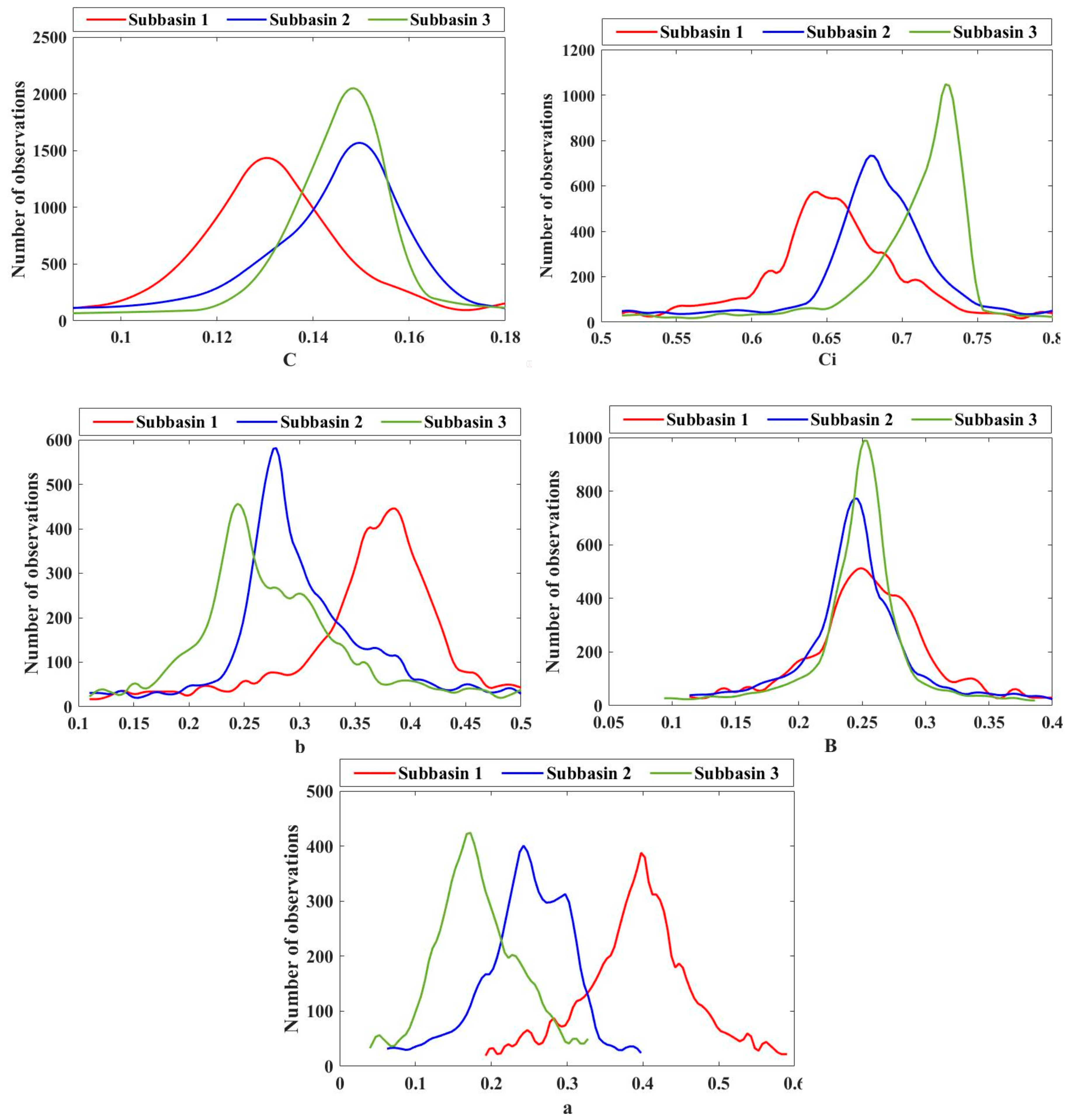
The parameter sets obtained based on uniform distribution were input into the model for the model uncertainty analysis. Figure 5 presents the distribution curves of parameters of the three sub-basins simulated by the modified GXAJ model. According to the figure, the distributions of different parameters at different sub-basins are different, but they are all unimodal. The C parameter of Sub-basin 1 has the largest value, while the C values of Sub-basins 2 and 3 are close. This is due to the low vegetation coverage in Sub-basin 1, and the higher vegetation coverage in Subbasins 2 and 3. Regarding the C_i parameters, the values of Subwatersheds 1, 2, and 3 decreased successively. This may be related to the differences in elevation between the basins. The value of b is mainly related to the area of the basin, which increases with area, and vice versa [26,27]. Here, the distribution of B values is relatively close, with little difference in each subwatershed. Parameter a is related to the average basal area of plant stem. The simulation parameters showed that the values of Subwatersheds 3, 2, and 1 increase successively.

Then, the uncertainty area was analyzed by using runoff simulation results with a likelihood function value greater than 65% [33]. Figure 6 shows the prediction interval, the interval means, and observed values of the three sub-basins. The corresponding evaluation parameters (average relative length (ARIL), average asymmetry degree (AAD), and average deviation amplitude (ADA)) were calculated for quantitative analysis (

Table 4. Comparison of uncertainty parameters for the analyzed simulation conditions.

Uncertainty Parameter	Catchment
	Sub-Basin 1	Sub-Basin 2	Sub-Basin 3
average relative length (ARIL)	0.265	0.513	0.267
average asymmetry degree (AAD)	0.300	0.324	0.298
average deviation amplitude (ADA)	285.878	406.498	108.610

). It can be seen from the figure that the uncertainty of Subwatersheds 1 and 3 was small, and their prediction intervals were narrow. However, the uncertainty of Subwatershed 2 was large, and its prediction interval was wide. As can be seen from Table 2, the ARIL value of Subwatershed 2 was up to 0.5, and the model was shown to be uncertain, so the applicability of the model in this region needs to be strengthened.

5.3. Annual Water Budget Simulated by the Modified Xinanjiang Model

The water balance components of the three sub-basins are shown in

Table 5. The water balance components of the three sub-basins.

Watershed	Year	Precipitation	Storage Change	Modeled Annual Actual Evaporation	Measured Discharge
Sub-basin 1	mean annual (mm)	461.50	−1.08	258.63	201.90
	σ/Mean	0.23	-	0.09	0.38
	correlation with Precipitation	1.00	0.85	0.41	0.81
Sub-basin 2	mean annual (mm)	753.16	−1.40	338.12	446.16
	σ/Mean	0.20	-	0.07	0.40
	correlation with Precipitation	1.00	0.66	0.64	0.95
Sub-basin 3	mean annual (mm)	909.76	1.62	422.21	479.53
	σ/Mean	0.27	-	0.07	0.46
	correlation with Precipitation	1.00	0.62	0.59	0.94

. Sub-basin 3 had the highest values of measured mean annual precipitation (MMAP), streamflow, and simulated evapotranspiration, and Sub-basin 1 had the lowest values. The interannual variation (standard deviation (σ)/annual mean) of MMMP for each sub-basin ranged from 0.2 to 0.27, while that of the measured streamflow was the biggest and ranged from 0.38 to 0.46. The interannual variation of the simulated evapotranspiration was the smallest. The precipitation was shown to have a great influence on the storage changes in the semi-arid and semi-humid regions. The correlation coefficient between the annual storage change and the precipitation for Sub-basin 1 was significantly high (0.85), whereas it was low for Sub-basin 2 and Sub-basin 3. On the contrary, the correlation between AE and the precipitation for Sub-basin 1 was the lowest, with a value of 0.41. This value is far lower than those of the other two sub-basins. The correlation coefficients between the measured streamflow and the precipitation for the three sub-basins were 0.81, 0.95, and 0.94 for Sub-basins 1, 2, and 3, respectively. Because the study did not examine groundwater as a factor, the annual ground water storage was considered to be unchanged.

5.4. Seasonal Variation of the Evapotranspiration and the Soil Moisture

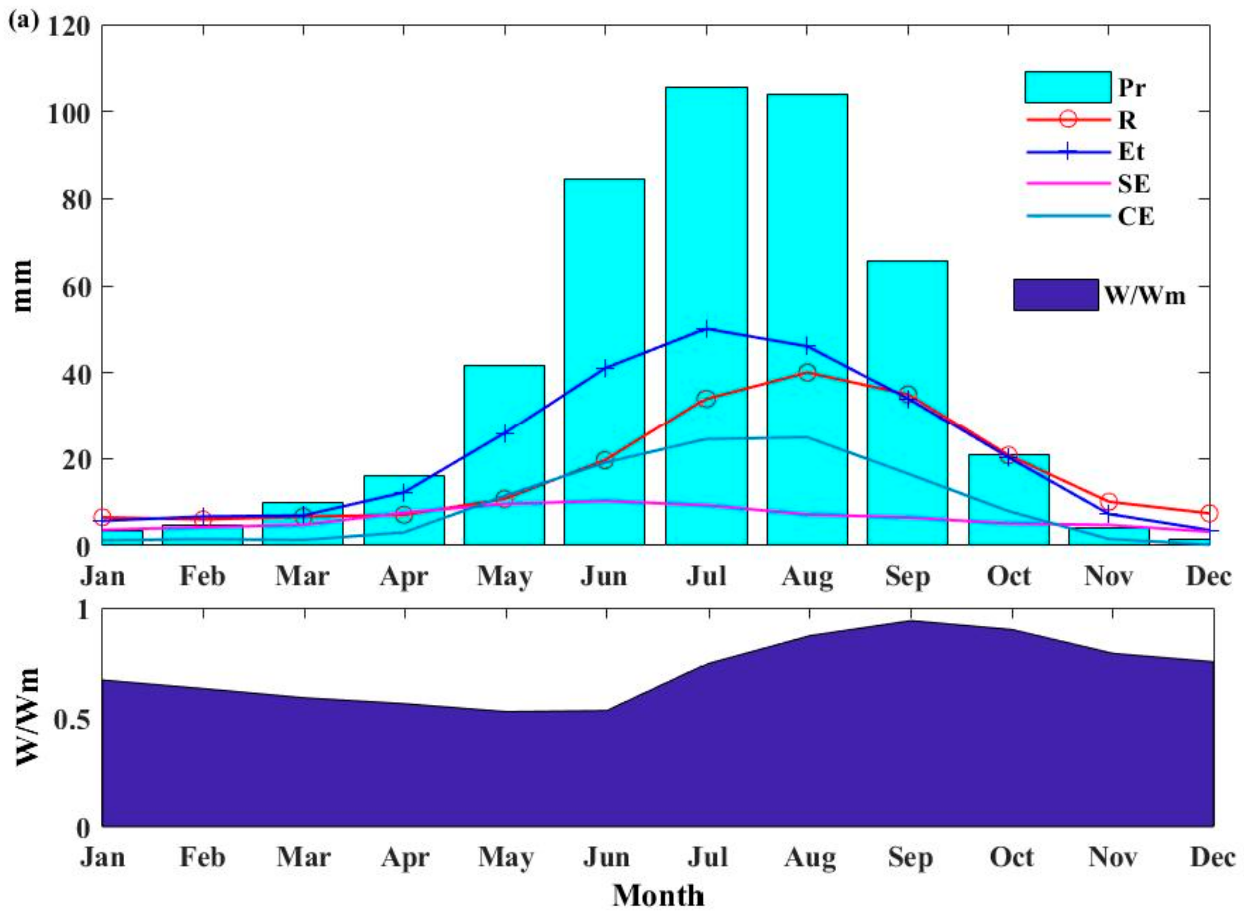
The series of monthly precipitation, runoff, evapotranspiration (E_t), CT, SE, and the ratio of the mean tension water storage (W) to tension water capacity (W_M) are shown in Figure 7a–c. The maximum monthly precipitation levels of each sub-basin were 105, 155, and 206 mm, respectively. The curve of the runoff hydrograph appeared 1 month after the one of the rainfall in the wet season. The annual evapotranspiration was larger than the runoff at Sub-basin 1 and smaller for Sub-basin 2 and Sub-basin 3. During the period of May to October, the CT exceeded the SE markedly due to the dense vegetation canopy and vice versa. This result shows that the value of W/W_M (taken as the soil moisture content) is high from July to November, coinciding with the summer monsoon, while the value of W/W_M is low from March to May because of the vegetation growth and infrequent rain. Compared to Sub-basin 1, the monthly soil water contents of Sub-basin 2 and Sub-basin 3 were higher. However, even in the rainy season of the humid Sub-basin 3, the soil was not saturated every day. Therefore, it is necessary to take both IER and SER into account in the rainfall runoff process.

5.5. Spatial Patterns of the Annual Precipitation and Evapotranspiration

Figure 8a–c show the spatial heterogeneity of the annual average precipitation, evapotranspiration, and fraction of evapotranspiration to precipitation (E/P). The land cover, elevation, and mean annual temperatures are shown in Figure 6d,e. The annual precipitation level indicated a significant spatial heterogeneity in the basin. The greatest amount of rain fell in the valley area of Sub-basin 3, which is the outlet of the total basin. The smallest precipitation occurred in the north of Sub-basin 1, which is located in the Tibetan Plateau. In the intermediate region of the Jinshajiang Basin, the precipitation of Sub-basin 2 was larger than that of Sub-basin 1, even in similar topographies.

Evapotranspiration is controlled by many factors, such as the air temperature, precipitation, speed, incoming shortwave radiation, and land cover. Sub-basin 3 evaporates the most water annually as a result of the high mean annual temperature, heavy rainfall, lower latitude (higher incoming shortwave radiation), higher vegetation coverage, and a relatively high speed (not shown). For Sub-basin 1, however, the exception is the upper area, which evaporates more water than the downstream area. The upper area of Sub-basin 1 has less precipitation, a lower mean annual temperature, a lower speed, and sparse vegetation, whereas the high altitude enhances the incoming shortwave radiation, promoting evapotranspiration. For different vegetation types, the mean annual evapotranspiration showed significant differences across the basin, ranging from 189.81 to 585.45 mm/year. Forest and woodland, which are mainly concentrated in the mid-low reaches of the Jinshajiang River, evaporate most, with a mean value of 485.6 mm/year. The cropland scattered in Sub-basin 2 and Sub-basin 3 ranked second-high for evaporation, at 392.3 mm/year. The shrubland (shrubby deserts) and grassland, which are mainly concentrated in the upper stream ranks, had the lowest evaporation, with average values of 289.4 mm and 275.9 mm, respectively. The E/P represents the degree of drought. The pattern of the E/P values of different vegetation types was different from that of evapotranspiration. The shrub-covered land was shown to have a shortage of water, with an E/P of 83%. The region of forest and grassland is humid, and the E/P values were shown to be 54% and 53%, respectively. The region of cropland was shown to be the moistest, with an E/P of 48%.

6. Conclusions

A modified form of the distributed GXAJ model considering the infiltration excess and saturation excess runoff mechanisms coupled to a TSPE model was established to quantify the water balance and analyze the spatiotemporal patterns of precipitation, evapotranspiration, and soil moisture of three sub-basins in the Jinshajiang River basin. In the flow routing module, the outflow is routed using the physical NMC method. A priori parameter estimation was used to obtain land use and land cover (LULC) data, vegetation data, soil data, and routing parameters. LAI data was obtained from the BNU MODIS LAI dataset.

The modified GXAJ model was developed and applied to simulate the daily runoff in the three sub-basins in the Jinshajiang River basin. The results demonstrated that the modified GXAJ model achieved satisfactory performance in the three sub-basins and especially improved the simulation results of the peak discharges of the flood, compared to the TSPE + GRAJ model.

The precipitation in the humid region mainly affects the evapotranspiration, soil storage, and discharge. The evapotranspiration in the semi-arid region is characterized by the combined effects of climatic factors and land cover, while there is a strong correlation between the soil storage as well as the discharge and precipitation. The evapotranspiration and E/P also differ for different types of vegetation. Forest and woodland evaporate the most water annually, cropland takes second place, and shrubland and grassland evaporate the least amounts of water. The desert shrub concentrated in the upper stream of the Jinshajiang River basin is dry with an E/P of 83%; the humid middle and lower Jinshajiang region are covered with forest and grassland with E/P values of 54% and 53%, respectively. Cropland is rich in water resources with an E/P of 48%.

In the present model, the freeze–thaw process was not taken into account, which led to some discrepancies in the results for the cold season. The frozen soil and snow module will be considered in our future studies to enhance the ability of simulating the runoff generation in the outlet of the basin. Furthermore, more spatiotemporal data, such as groundwater data, ET data, and snow data, are needed from remote sensing or field measurements to test the results and improve the understanding of the interior ungauged region. The integrated model may also be applied for the assessment of the effects caused by climate change on the streamflows under different Representative Concentration Pathway (RCP) scenarios.

References

- Hu, C.; Guo, S.; Xiong, L.; Peng, D. A modified Xinanjiang model and its application in northern China. Nord. Hydrol. 2005, 36, 175–192. [Google Scholar] [CrossRef]
- Zhao, R.; Liu, X. The Xinanjiang model. In Computer Models of Watershed Hydrology; Singh, V.P., Ed.; Water Resources Publications: Littleton, CO, USA, 1995. [Google Scholar]
- Gan, T.Y.; Dlamini, E.M.; Biftu, G.F. Effects of model complexity and structure, data quality, and objective functions on hydrologic modeling. J. Hydrol. 1997, 192, 81–103. [Google Scholar] [CrossRef]
- Jayawardena, A.; Zhou, M. A modified spatial soil moisture storage capacity distribution curve for the Xinanjiang model. J. Hydrol. 2000, 227, 93–113. [Google Scholar] [CrossRef]
- Zhang, D.; Zhang, L.; Guan, Y.; Chen, X.; Chen, X. Sensitivity analysis of Xinanjiang rainfall–runoff model parameters: a case study in Lianghui, Zhejiang province, China. Hydrol. Res. 2012, 43, 123–134. [Google Scholar] [CrossRef]
- Xu, H.; Xu, C.; Chen, H.; Zhang, Z. Assessing the influence of rain gauge density and distribution on hydrological model performance in a humid region of China. J. Hydrol. 2013, 505, 1–12. [Google Scholar] [CrossRef]
- Yao, C.; Li, Z.; Bao, H.; Yu, Z. Application of a developed Grid-Xinanjiang model to Chinese watersheds for flood forecasting purpose. J. Hydrol. Eng. 2009, 14, 923–934. [Google Scholar] [CrossRef]
- Yao, C.; Li, Z.; Yu, Z.; Zhang, K. A priori parameter estimates for a distributed, grid-based Xinanjiang model using geographically based information. J. Hydrol. 2012, 468, 47–62. [Google Scholar] [CrossRef]
- Ren, G.; Guo, J. Change in pan evaporation and influential factors over China:1956–2000. J. Nat. Resour. 2006, 21, 31–44. (In Chinese) [Google Scholar]
- Wang, Y.; Liu, B.; Zhai, J.; Su, B.; Luo, Y.; Zhang, Z. Relationship between potential and actual evaporation in Yangtze River Basin. Adv. Clim. Chang. Res. 2011, 6, 393–399. (In Chinese) [Google Scholar]
- Penman, H.L. Natural evaporation from open water, hare soil and grass. Proc. R. Soc. Lond. Ser. A 1948, 193, 120–145. [Google Scholar] [CrossRef]
- Monteith, J.L. Evaporation and the Environment, the State and Movement of Water in Living Organisms; Cambridge University Press: London, UK, 1965; pp. 205–234. [Google Scholar]
- Allen, R.G.; Pereira, L.S.; Raes, D.; Smith, M. Crop evapotranspiration. In Food and Agriculture Organisation Irrigation and Drainage Paper 56; Food and Agriculture Organization: Rome, Italy, 1988. [Google Scholar]
- Choudhury, B.J.; Monteith, J.L. A four-layer model for the heat budget of homogeneous land surfaces. Q. J. R. Meteorolog. Soc. 1988, 114, 373–398. [Google Scholar] [CrossRef]
- Yuan, F.; Ren, L.; Yu, Z.; Xu, J. Potential evapotranspiration computation using a two-source method for the Xin’anjiang hydrological model. J. Hydrol. Eng. 2008, 13, 305–316. [Google Scholar] [CrossRef]
- Holtan, H.N. A Concept for Infiltration Estimates in Watershed Engineering. Agric. Res. 1961, 150, B16–B25. [Google Scholar]
- Getirana, A.C.V.; Boone, A.; Peugeot, C. Evaluating LSM-based water budgets over a west African basin assisted with a river routing scheme. J. Hydrometeorol. 2014, 15, 2331–2346. [Google Scholar] [CrossRef]
- Gangopadhyay, M.; Uryvaev, V.A.; Oman, M.H.; Nordenson, T.J.; Harbeck, G.E. Measurement and Estimation of Evaporation and Evapotranspiration; WMO: Geneva, Switzerland, 1966. [Google Scholar]
- Liu, X.; Ren, L.; Yuan, F.; Singh, V.P.; Fang, X.; Yu, Z.; Zhang, W. Quantifying the effect of land use and land cover changes on green water and blue water in northern part of China. Hydrol. Earth Syst. Sci. 2009, 13, 735–747. [Google Scholar] [CrossRef] [Green Version]
- MO, X.; LIN, Z.; LIU, S. An improvement of the dual-source model based on Penman-Monteith formula. J. Hydrol. Eng. 2000, 5, 6–11. [Google Scholar]
- Xu, J.; Ren, L.; Ruan, X.; Liu, X.; Yuan, F. Development of a physically based PDSI and its application for assessing the vegetation response to drought in northern China. J. Geophys. Res. Atmos. 2012, 117, D8. [Google Scholar] [CrossRef]
- Jinshajiang River Basin in China. Data Center for Resources and Environmental Sciences, Chinese Academy of Sciences (RESDC). Available online: http://www.resdc.cn/data.aspx?DATAID=141 (accessed on 12 May 2016).
- Changjiang & Southwest Rivers Water Resources Bulletin, Changjiang Water Resources Commission of the Ministry of Water Resources. Available online: http://www.cjw.gov.cn/zwzc/bmgb/ (accessed on 12 May 2016). (In Chinese)
- Fu, B.; Lu, Q. Atlas of Microclimate over Shanxi Basin; Nanjing University Press: Nanjing, China, 1990. (In Chinese) [Google Scholar]
- Song, X.; Kong, F.; Zhan, C.; Han, J.; Zhang, X. Parameter identification and global sensitivity analysis of Xin’anjiang model using meta-modeling approach. Water Sci. Eng. 2013, 6, 1–17. [Google Scholar]
- Zhao, R.; Wang, P. Parameter analysis for Xinanjiang model. J. China Hydrol. 1988, 6, 2–9. Available online: http://www.cnki.com.cn/Article/CJFDTotal-SWZZ198806000.htm (accessed on 12 May 2016). (In Chinese).
- Zhao, R.; Wang, P.; Hu, F. Relations between parameter values and corresponding natural conditions of Xinanjiang model. J. Hohai Univ. 1992, 20, 52–59. (In Chinese) [Google Scholar]
- Shu, C.; Liu, S.; Mo, X.; Liang, Z.; Dai, D. Uncertainty analysis of Xinanjiang model parameter. Geogr. Res. 2008, 27, 343–352. (In Chinese) [Google Scholar]
- Anderson, R.; Koren, V.; Reed, S. Using SSURGO data to improve Sacramento Model a priori parameter estimates. J. Hydrol. 2006, 320, 103–116. [Google Scholar] [CrossRef]
- Koren, V.; Smith, M.; Wang, D.; Zhang, Z. Use of Soil Property Data in the Derivation of Conceptual Rainfall–Runoff Model Parameters, 2000. Available online: http://www.nws.noaa.gov/oh/hrl/modelcalibration/3.%20%20A%20priori%20model%20parameters/ams_2000_koren_soils_parameters.pdf (accessed on 12 May 2016).
- Duan, Q.Y.; Gupta, V.K.; Sorooshian, S. Shuffled complex evolution approach for effective and efficient global minimization. J. Optim. Theory Appl. 1993, 76, 501–521. [Google Scholar] [CrossRef]
- Duan, Q.; Sorooshian, S.; Gupta, V.K. Optimal use of the SCE-UA global optimization method for calibrating watershed models. J. Hydrol. 1994, 158, 265–284. [Google Scholar] [CrossRef] [Green Version]
- Nash, J.E.; Sutcliffe, J.V. River flow forecasting through conceptual models, Part-I: A discussion of principles. J. Hydrol. 1970, 10, 282–290. [Google Scholar] [CrossRef]
- Walega, A.; Ksiazek, L. Influence of rainfall data on the uncertainty of flood simulation. Soil Water Res. 2016, 11. [Google Scholar] [CrossRef]
- Blasone, R.S. Parameter Estimation and Uncertainty Assessment in Hydrological Modelling. Ph.D. Thesis, Technical University of Denmark, Copenhagen, Denmark, August 2007. [Google Scholar]
- Jin, X.; Xu, C.; Zhang, Q.; Singh, V.P. Parameter and modeling uncertainty simulated by GLUE and a formal Bayesian method for a conceptual hydrological model. J. Hydrol. 2010, 383, 147–155. [Google Scholar] [CrossRef]
- Xiong, L.; Wan, M.; Wei, X. Indices for assessing the prediction bounds of hydrological models and application by generalized likelihood uncertainty estimation. Hydrol. Sci. J. 2009, 54, 852–871. [Google Scholar] [CrossRef]