Development of RiverBox—An ArcGIS Toolbox for River Bathymetry Reconstruction

Department of Hydraulic and Sanitary Engineering, Poznan University of Life Sciences, ul. Wojska Polskiego 28, 60-637 Poznan, Poland
Water 2018, 10(9), 1266; https://doi.org/10.3390/w10091266
Submission received: 29 August 2018
/
Revised: 13 September 2018
/
Accepted: 13 September 2018
/
Published: 17 September 2018
(This article belongs to the Special Issue Applications of Remote Sensing and GIS in Hydrology)
Abstract
:The main purpose of the present research is to develop software for reconstruction of the river bed on the basis of sparse cross-section measurements. The tools prepared should support the process of hydrodynamic model preparation for simulation of river flow. Considering the formats of available data and the requirements of modern modeling techniques, the prepared software is fully integrated with the GIS environment. The scripting language Python 2.7 implemented in ArcGIS 10.5.1 was chosen for this purpose. Two study cases were selected to validate and test the prepared procedures. These are stream reaches in Poland. The first is located on the Warta river, and the second on the Ner river. The data necessary for the whole procedure are: a digital elevation model, measurements of the cross-sections in the form of points, and two polyline layers representing an arbitrary river centerline and river banks. In the presented research the concept of a channel-oriented coordinate system is applied. The elevations are linearly interpolated along the longitudinal and transversal directions. The interpolation along the channel is implemented in three computational schemes linking different tools available in ArcGIS and ArcToolbox. A simplified comparison of memory usage and computational time is presented. The scheme linking longitudinal and spatial interpolation algorithms seems to be the most advantageous.
1. Introduction
The main problem analyzed in the present research is the reconstruction of river channel bathymetry on the basis of sparse measurements. It is assumed that measurements are taken in typical ways for river engineering, such as bathymetric surveys in selected cross-sections. The importance of this problem is growing, with increasing interest in and application of one-dimensional as well as two-dimensional river hydrodynamic models. The development of such a tool has to reflect the requirements and needs of the application area to model flow and other processes in rivers. One of the most important needs is the integration of hydrodynamic modeling with the GIS environment. Hence, the research done is presented in the form of a toolbox consisting of methods supporting the process of river bathymetry reconstruction. The toolbox is called RiverBox and it is fully integrated with one of the most popular GIS environments, ArcGIS, developed by the company Esri (Redlands, CA, USA).
The reconstruction of river bathymetry is not a new problem, but interest in this area has begun to grow in recent times. Two of the first papers were published by Tate et al. [1] and Goff and Nordfjord [2]. These works, like the majority of the literature in this field, are based on a channel-oriented coordinate system. This means that the coordinate system consists of longitudinal and transversal coordinates. The first is assigned to the river centerline or thalweg. The second is perpendicular to the first in most cases. Such an approach is an application of an older concept related to the generation of boundary-fitted numerical grids [3]. The two mentioned publications used very simple approaches. The main idea of the former is based on linking the GIS techniques and the well-known hydrodynamic modeling package HEC-RAS (Hydrologic Engineering Center—River Analysis System, HEC, Davis, CA, USA). The fundamental element is an arbitrary determination of the river centerline. The cross-section shape does not depend on other spatial information, e.g., location of banks. Although it is quite a simple approach, even today it is used widely in such modeling systems as HEC-RAS and MIKE 11 (DHI, Hørsholm, Denmark). The procedure developed in the second paper uses more information for bed reconstruction. This involves the river centerline, the bank lines, and additional track lines. All the lines are determined arbitrarily. The interpolation of elevations is done along the track lines including the centerline and the banks. The whole procedure of track line preparation is time consuming.
These two approaches are improved and extended in the papers published by Merwade and co-authors [4,5]. The main idea presented there is based on the linking of the longitudinal coordinate with the stream thalweg. The problem is that the thalweg is not determined a priori. It has to be calculated iteratively with improvement of the interpolation. This approach may extend the computational time. The extension of this concept was published in Merwade’s next papers [6,7] and finally applied as an ArcGIS plug-in [7,8,9,10,11] working with older versions of ArcGIS (up to 10.3).
The problem of river bed reconstruction has also been studied by other researchers. In the paper written by Legleiter and Kyriakidis [12] a very interesting and fairly complex procedure for the transformation of geographic and channel-oriented coordinates is described. Schäppi et al. [13] also presented an original approach to the problem of coordinate transformation. In most cases the longitudinal coordinate is determined first, and then the transversal coordinate is calculated. Schäppi and co-authors developed a scheme where this direction is reversed. Additionally, the coordinate lines do not need to be orthogonal. The concepts presented by Merwade et al. [4] and Schäppi et al. [13] were implemented by Bogusz et al. [14] and compared with an interpolation procedure available in MIKE 11. As mentioned above, the latter approach is similar to the basic method described by Tate et al. [1]. A slightly different concept was presented by Kardos [15]. The combination of algebraic mesh, linear interpolation along mesh lines, and spatial inverse distance interpolation is applied there. The most modern concept based on the discussed ideas is presented by Caviedes-Voullième et al. [16]. In this research the thalweg plays the role of the longitudinal axis. The procedure is based on generation of intermediate cross-sections and transformation of the elevations interpolated in a cross-section to the 2D plane.
For some time, more sophisticated approaches have been presented in scientific journals. For example, Farina et al. [17] applied the entropy principle for reconstruction of the bed. In turn, Zhang et al. [18] developed a specific spatial interpolation method for this problem. The method is known as shortest temporal distance. It uses specific metrics to adjust the whole procedure to the channel-oriented problem. Finally, Lai et al. [19] applied concepts borrowed once again from Thompson et al. [3]. They applied an elliptic equation to generate an orthogonal and boundary-fitted grid along the channel. All these three mentioned approaches are very interesting, but their resilience to data sparseness has not been tested. According to the present author’s expectations, the uncertainty of the data caused by sparse measurements may be the reason to avoid sophisticated approaches and focus on simpler techniques.
The main purpose of the present research is to develop a toolbox including methods supporting reconstruction of river bathymetry. The river bed bathymetry should be created as a Digital Elevation Model (DEM). It should be easily linked with a DEM of the surrounding area, completing this layer with appropriate information about bed elevations. The toolbox is prepared as a set of methods fully integrated with the ArcGIS environment. The Python 2.7 scripting language is used, because this programming environment is also integrated with the current version of ArcGIS (10.5.1). The main idea applied is interpolation of the river elevations in a channel-oriented coordinate system. The main concern is the accuracy and efficiency of the methods applied. The problem of computational speed is crucial in cases of fairly slow scripting languages. To overcome this drawback, a specific hybrid method linking longitudinal and spatial interpolations is proposed and tested.
2. Materials
2.1. Chosen Case Study
Two river reaches were chosen for the tests. The selection was done considering their lengths, variability of geometric properties, and availability of data. The analyzed channels are: (1) the reach of the Warta river near the town of Wronki in the western part of Poland and (2) the downstream part of the Ner river in the central part of Poland.
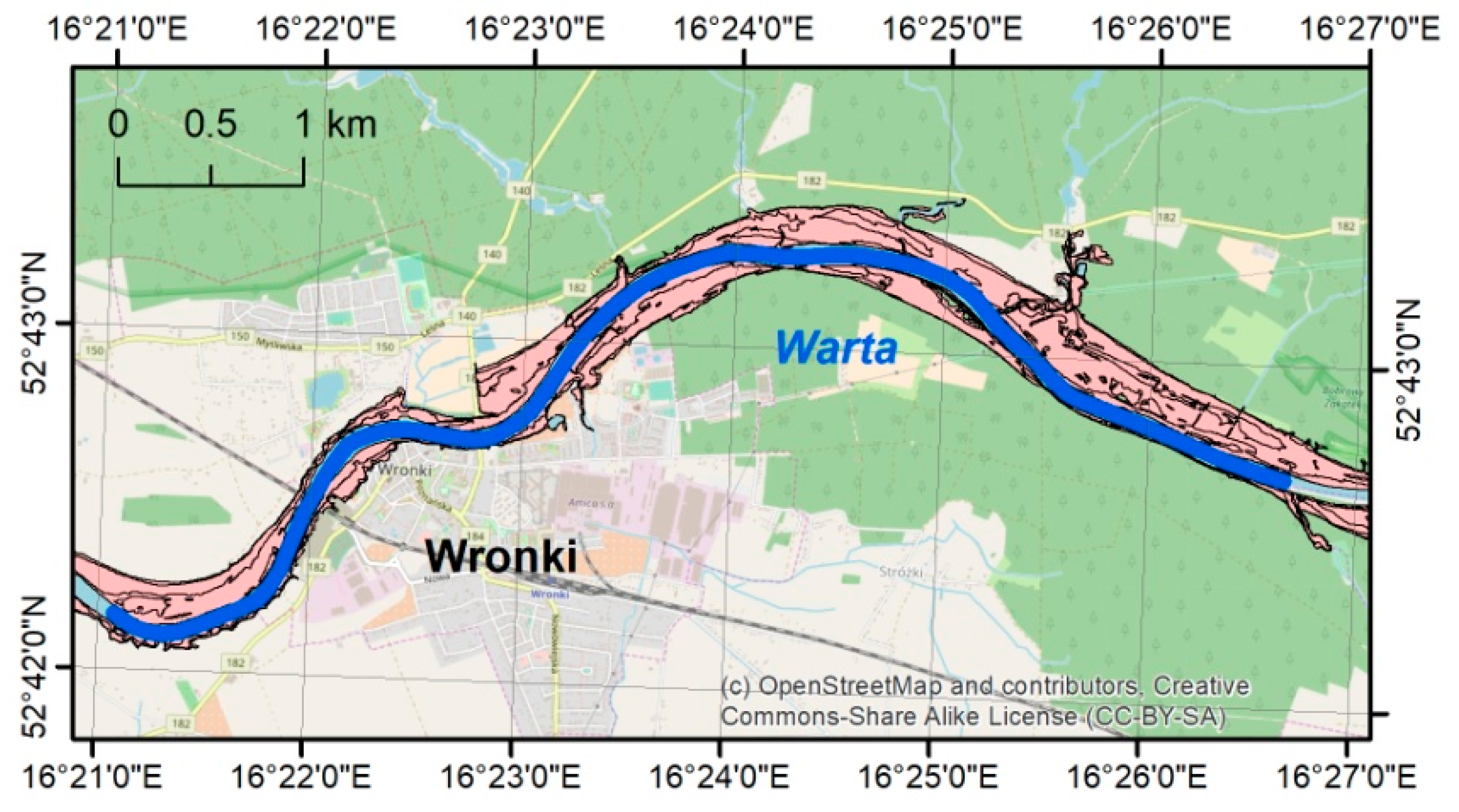
The Warta river is a right tributary of the Oder river, which flows along the border between Poland and Germany. The Warta is fourth in the list of the longest rivers in Poland. The length of the first reach chosen is fairly short. It measures approximately 7.6 km. The average width of the channel is 70 m. Along this short reach the width changes slightly. The average depth is about 1.5–1.6 m. In the town of Wronki the gauge station is installed. It enables monitoring of the water stages and assessment of discharges. The mean discharge in this part of the Warta river is 124.7 m3/s. For the determination of inundation areas and flood hazard maps the extreme discharges representing 10-, 100- and 500-year floods were used. Their values are 560 m3/s, 928 m3/s, and 1211 m3/s, respectively. In 2016 these data were bought from the Polish Institute of Meteorology and Water Management (IMGW—Polish Instytut Meteorologii i Gospodarki Wodnej). All quoted hydrological characteristics are estimated on the basis of observations and data measured in the period 1971–2014. The whole reach is denoted with a blue line in Figure 1. The pink area represents the inundation area for a 100-year flood.
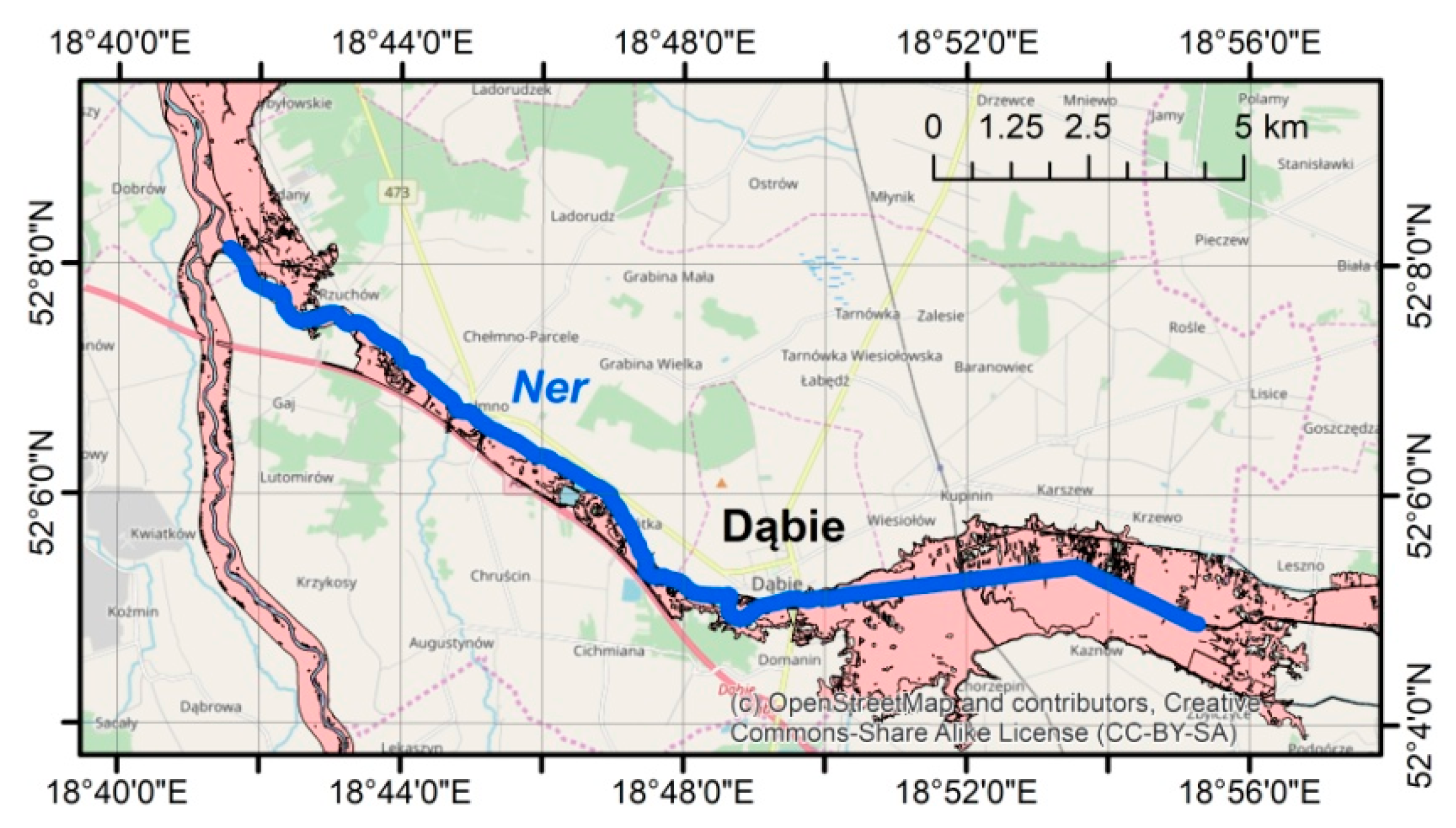
The Ner river is the right tributary of the Warta river. Although this reach is about 19 km long, the average width of the channel is much smaller than before, and it equals about 20 m. The changes of the width along the channel vary from over 12 m to 30 m or more. The average depth is about 1 m. The only gauge station in this reach is located in the middle, in the town of Dąbie. This equipment enables observation of water stages and assessment of discharges. The average discharge is 10.93 m3/s. The extreme values are as follows: for a 10-year flood 129.72 m3/s, for a 100-year flood 191.73 m3/s, and for a 500-year flood 230.93 m3/s [20]. All these values are assessed on the basis of data observed during the period 1961–2013. The modeled reach is presented as a blue line in Figure 2. As before, the pink areas denote the flood inundation for a 100-year event.
2.2. Available Data for Bathymetry Reconstruction
There are three sets of data necessary for interpolation of the river bed. These are: (1) the basic digital elevation model (DEM); (2) the measurements of the river cross-sections; and (3) two polyline layers representing the river centerline and river banks. Only the last element has to be prepared manually by the user.
Two DEMs are applied in the presented research. The first represents the area surrounding the reach of the Warta river near the town of Wronki. The second is used for tests with the reach of the Ner river. Both of them are obtained from Head Office of Geodesy and Cartography (GUGiK—Polish Główny Urząd Geodezji i Kartografii). Their spatial and vertical resolutions are the same. The size of the cell is 1 m in each direction. The vertical resolution is 15 cm. Their file sizes are 467 MB and 1340 MB, respectively. The sizes of tables expressed as column times rows are 12,995 × 9421 in the first case and 25,713 × 13,965 in the second. Hence, the total areas are 122 km2 and 359 km2, respectively. The nonempty areas are smaller, equaling 78 km2 and 297 km2, respectively.
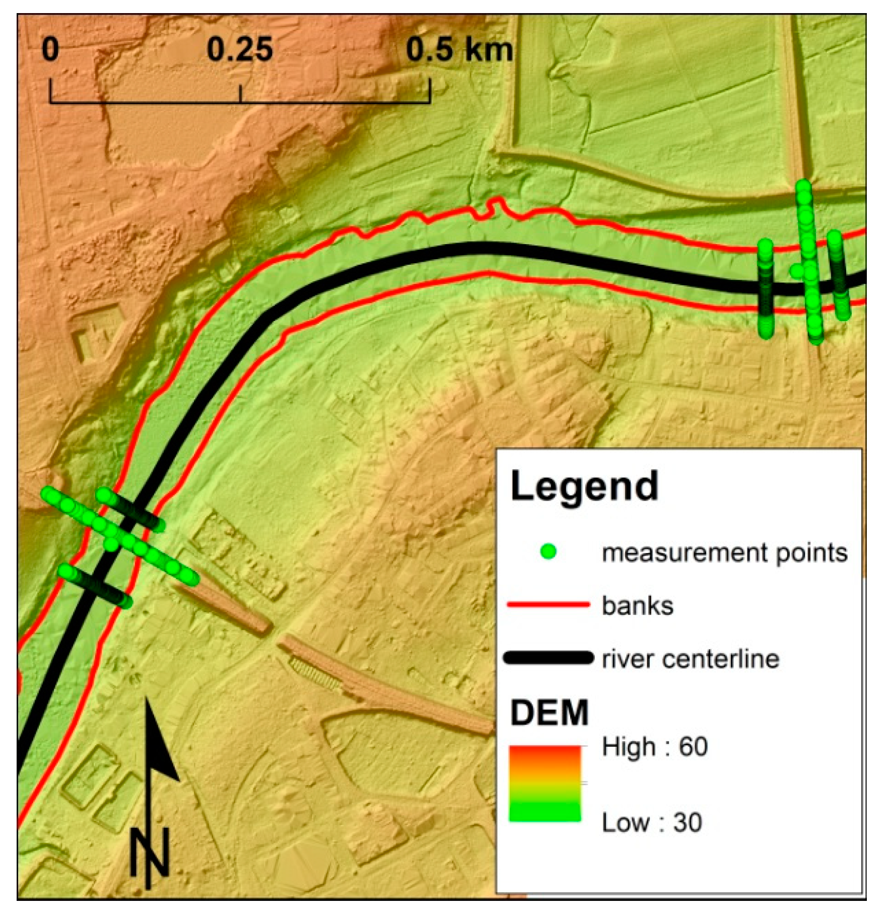
Example data are shown in Figure 3. The DEM is shown in green-red colors and covered with a transparent hillshade layer. The black line represents the river centerline. The red lines are used for reconstruction of the river banks. The measurement points are denoted as green dots. The number of points is not small, but their location disables application of standard spatial interpolation methods, e.g., those available in ArcToolbox (Redlands, CA, USA).
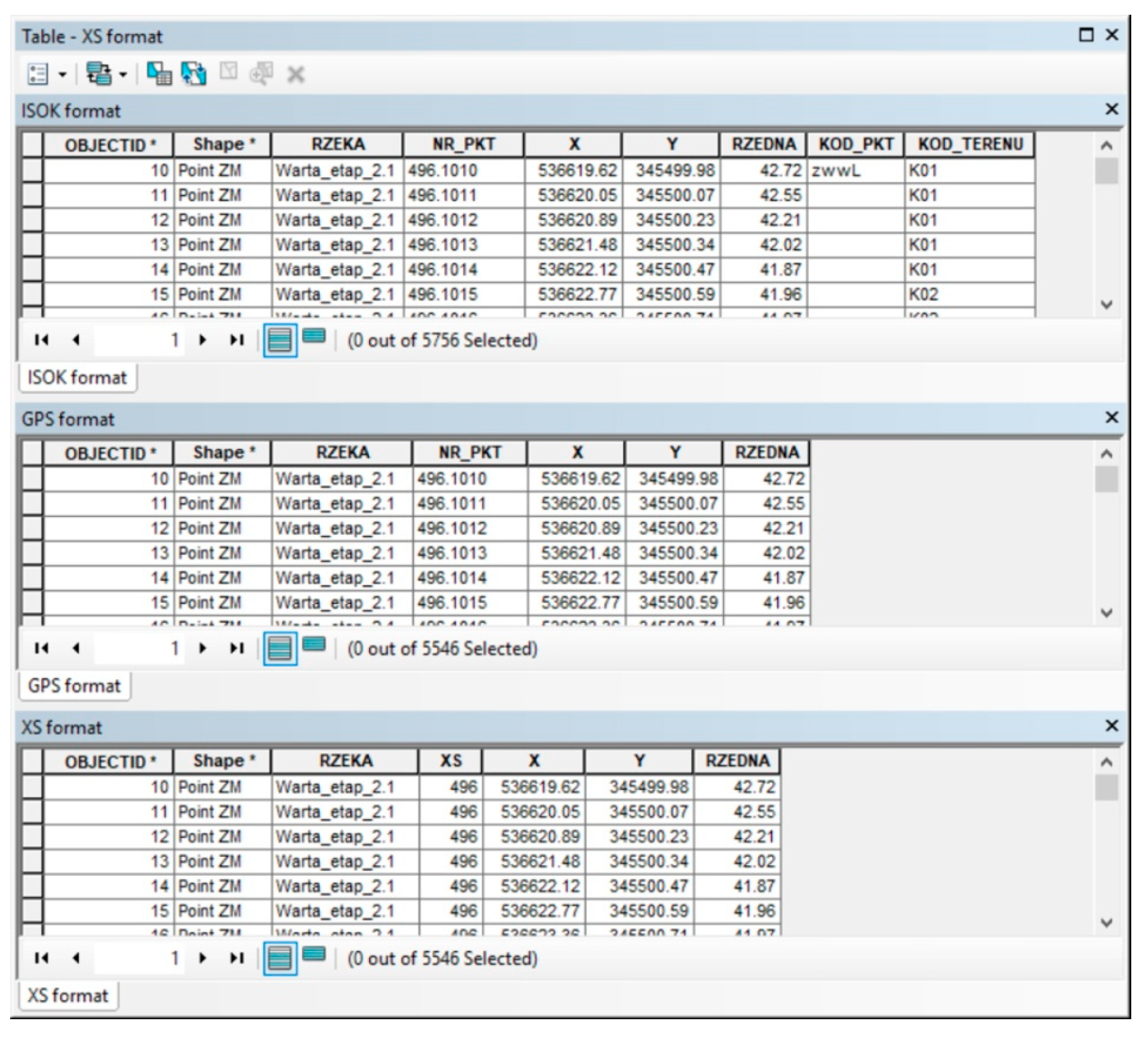
At the current stage of toolbox development, the measurements of cross-sections may have one of three forms. The differences between these forms are hidden in the tables of attributes. Examples are shown in Figure 4. The basic form consists of the points from GPS measurements. They are referred to here as GPS points. In such a case the table of attributes has to contain the number of measurement points and the elevation at each point. The number of points has the format “XS.pnt”, where “XS” is the number of cross-sections and “pnt” is the number of points. The names of the attributes are not known a priori. The user has to choose appropriate attributes (columns in Figure 4) before the tool is run. The more developed format is called the ISOK format. It is referred to here as “ISOK points”. This format was used for measurements in the ISOK project in Poland, as per the IT system of the Country’s Protection Against Extreme Hazards (ISOK—Polish Informatyczny System Osłony Kraju przed nadzwyczajnymi zagrożeniami). The EU Flood Directive was implemented as part of this system in Poland. In the case of the ISOK format the table of attributes includes the number of the point as “XS.pnt” and elevation as well. The names of the attributes are known a priori. These are “NR_PKT” (in Polish, meaning point number) and “RZEDNA” (in Polish, meaning elevation), respectively. The measurements in the ISOK project were also used for description of the hydro-structures’ shape. Hence, there is also information about the type of the point in the table of attributes. This column is denoted as “KOD_PKT” (in Polish, meaning code of points). The identification numbers located there may be used for selection of points before the interpolation. The additional attribute present in the ISOK points is “KOD_TERENU” (in Polish, meaning code of terrain). These values may be used further for determination of the roughness coefficients. The final and the simplest format is that of the XS points. In the table of attributes there is only information about the number of cross-sections and the elevation. Both attributes have to be indicated by the user.
Along the reach of the Warta river there are 11 cross-sections measured. The average distance between measurements is 756 m. The measurements near two bridges in the town of Wronki are spaced closer together. Their average distance apart is 52 m. On the other hand, the maximum distance between cross-sections is 1460 m. The average number of measurement points in a single cross-section is 136. The course of the river and its width give 0.66 km2 for bed interpolation. The average and the longest distance between interpolated cells and measurements are 160 m and 730 m, respectively.
The characteristics of the analyzed reach of the Ner river are slightly different. There are 35 measurement cross-sections along the reach. The average and maximum distances between measurements are 557 m and 2565 m, respectively. The difference between the average and the maximum is larger than in the previous case, which suggests greater non-uniformity of the measurements’ location. Near the structures, the distance between measurements is similar to the previous values. This time it is 59 m. The average number of measurement points per cross-section is much smaller, at nine points. Hence, the accuracy of the measurements is lower. Although the length of the reach is greater, the area for interpolation is smaller. In this case it is 0.41 km2. The reason for such differences in interpolation areas is the much smaller width of the channel in the second case. The estimated average distance between cells and measurements is smaller than before and equals 136 m, but the estimated maximum is 1283 m, which is about twice that in the previous case.
The last elements necessary for interpolation are two vector layers including polylines. The first should represent the river centerline. This layer does not include any specific attributes. The only requirement is that the direction of the line should be compatible with the direction of the flow in the river. The second layer should consist of the lines of the river banks—left and right, respectively. There should be a string attribute called “LineType”, where the type of the bank is denoted. The denotation should be “Left” or “Right”. The direction of lines should also be compatible with the direction of river flow.
2.3. Data for Validation Tests
The data used for direct interpolation in the two presented cases were measured as an element of the ISOK project, mentioned before. The field measurements of this project were taken in 2011–2012. The DEM obtained from GUGiK was created on the basis of LIDAR (Light Detection and Ranging) measurements made at the same time. To verify the results of the interpolation, other data are used. In the same reach, additional measurements were taken during 2015. Three cross-sections marked in Figure 9a were measured as preliminary work for design of the highway bridge located downstream of cross-section no. 4. The elevations were determined with a GPS device. Today, after 3 years, it is difficult to obtain information about this device and assess its accuracy. However, it is possible to compare measurements on the floodplains with the DEM obtained from CODGiK (Polish—Centralny Ośrodek Dokumentacji Geodezyjnej i Kartograficznej). The comparison of elevations was done at 59 points. The results showed that the mean error is about 31 cm and the maximum is 331 cm. The standard deviation is about 53 cm. The differences of greater than 50 cm between data from 2015 and the DEM used may be explained by the possible changes in terrain which could occur over the 3 years between two types of measurements. For example, there are differences in bank location, which may be the result of accidentally occurring bank instability caused by lateral erosion.
The measurements made in 2015 are used later for direct comparisons with interpolated bed elevations. The different times of the ISOK measurements and validation data may cause errors of another kind—those related to sediment processes and morphological changes of the bed. In fact, the period of 3 years is not long considering the scales of continuous sediment transport. Hence, the validation data may be good to assess overall correctness of the interpolation.
3. Methods
3.1. Basic Elements of the Algorithm
To create the presented toolbox, several mathematical methods from the area of computational geometry, linear regression, and approximation are implemented. These are the algorithm for determination of the straight-line equation, straight section cuts, points’ projections on lines, parallel and transversal lines, etc. However, the most important is the algorithm for interpolation in the channel-oriented coordinate system. This algorithm is presented below.
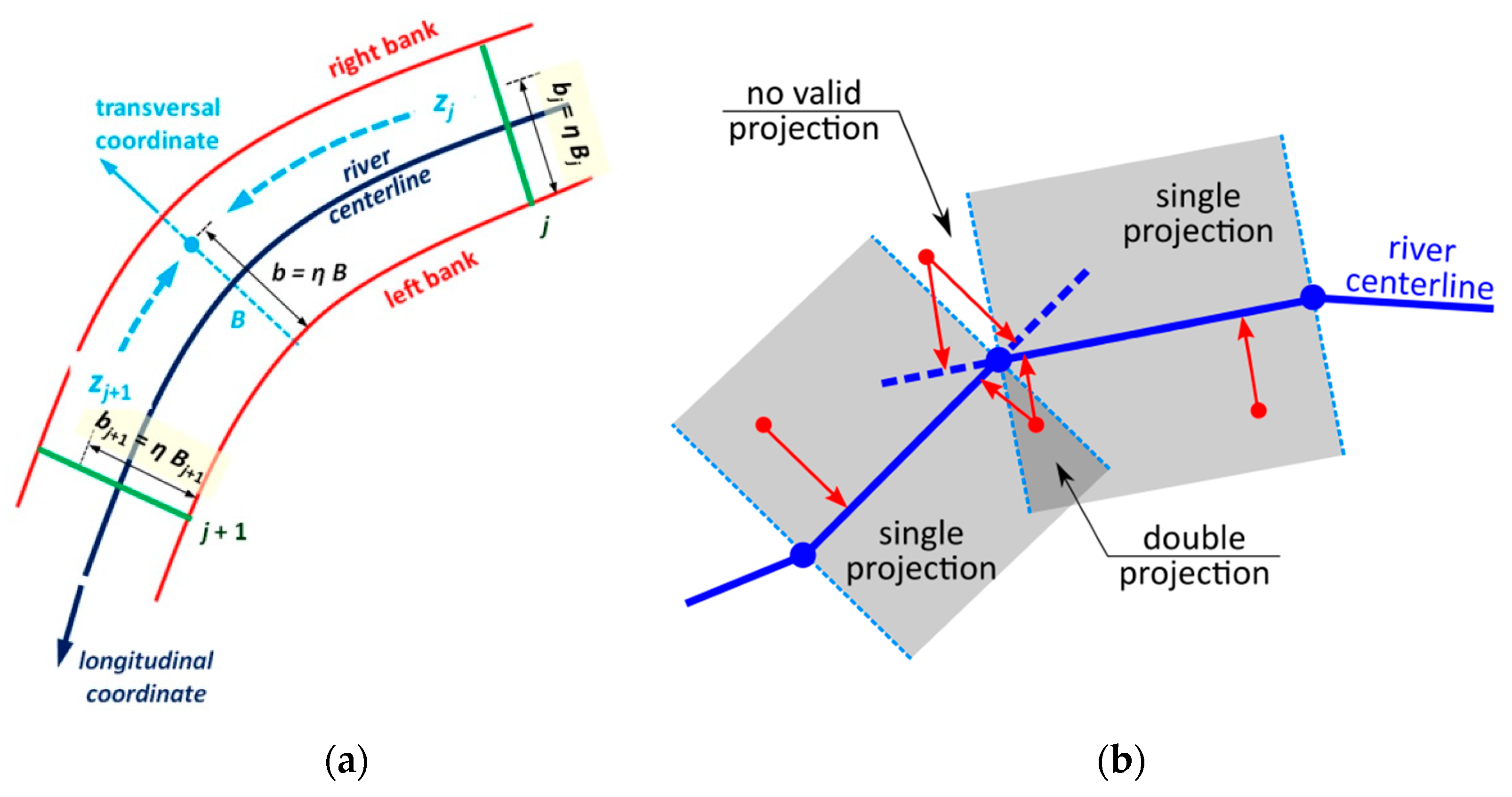
As discussed in the Introduction, the channel-oriented coordinate system is a system of two curvilinear axes. In the presented case the first is assigned to the arbitrary river centerline. The second represents cross-sections and it is locally normal to the longitudinal axis. The idea of such coordinates is presented in Figure 5a. The interpolation of bed elevations for each point located between banks is carried out in three steps:
- The point denoted as a blue dot is projected on the river centerline. The coordinates are determined in the following manner. The longitudinal one is calculated on the basis of linear referencing assigned to the centerline vertexes. The transversal coordinate is calculated as the relative distance of the point from the left bank measured along the projection direction.
- If the longitudinal coordinate is known, the two closest cross-sections with measurements can be found. One of them has to be located upstream and the second is found downstream of the river. As this stage, the measurements are represented by three-dimensional polylines of cross-sections. The vertexes of lines have four coordinates: namely spatial coordinates X and Y, elevation Z, and linear referencing along the cross-section M. The latter, M, is a transversal coordinate calculated as the relative distance from the left bank. In each selected cross-section the elevation is determined for the value of the transversal coordinate at the point projected previously (blue dot).
- The elevations determined in upstream and downstream cross-sections are used to linearly interpolate the elevation along the channel centerline. Finally, the elevation at the projected point is known.
The above basic procedure is easily applied for continuous river centerlines. However, the real centerlines are piecewise-linear curves. The projection is considered valid only if the projected point falls into the interior of the section where it is projected. Hence, there may be no valid projection zones, and double projection zones in the case of the piecewise-linear curve. They are shown in Figure 5b. Such cases require additional correction of the scheme described above. This problem was solved with a two-step procedure:
- For each vertex of the river centerline the cross-section is determined. The cross-section is perpendicular to the line connecting vertexes located upstream and downstream from the analyzed one. The longitudinal coordinate of this cross-section is the same as the coordinate determined for the analyzed vertex.
- The point located in the “no valid projection” or “double projection” zone is projected to the cross-section determined in step 1. For each such point the longitudinal coordinate is the same as the coordinate of the centerline node. Next, the transversal coordinate is calculated along this cross-section. The rule for calculation of the transversal is the same as shown previously.
Another important calculation problem is proper determination of cross-sections representing measurements. The well-known least square method [21] is applied assuming that the line of the cross-section is straight. For the sake of better accuracy, the coordinates are scaled in the range of the minimum and maximum in X and Y values. When the line is determined, its intersection with the river axis determines the location of the cross-section along the channel. The points where the line cuts the left and right banks are also determined. The measurement points are projected on the line and the relative distance from the left bank is calculated for each point. Then, the points are sorted according to this distance and the 3D line of measurement cross-section is created in such a way that each projection is a separate vertex. Each vertex has four coordinates, X, Y, Z, and M, as mentioned above. The basic parameter of the line is its position along the channel.
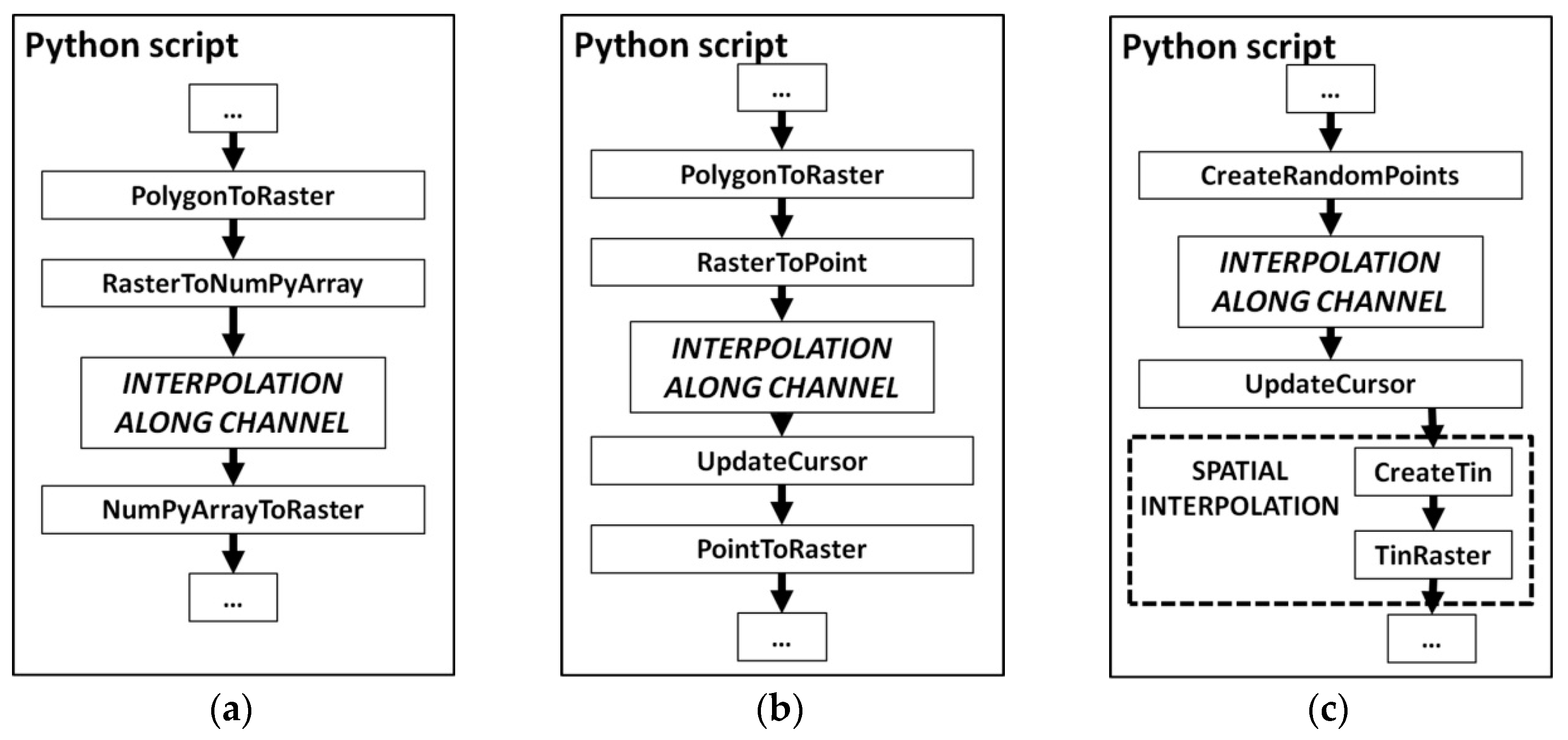
3.2. Applied Computational Schemes
The described basic techniques were applied in three computational schemes. The first scheme is presented in Figure 6a. The main computations start with transformation of the polygon covering the channel bed area to a single value raster. In general, the resolution of the raster should be the same as the resolution of the basic DEM. To avoid shifts between these two rasters, the origin point should also be set the same. This implies a large number of empty cells stored in the disk memory. Next, the raster is transformed into a NumPy array with the RasterToNumPyArray tool available in the ArcPy module of the Python environment linked with ArcGIS. The raster cells, empty and non-empty, are stored in the computer memory as array rows and columns. The interpolation along the channel described above is done for all non-empty array cells. Then the array is transformed to the raster with another tool called NumPyArrayToRaster. The mosaic techniques are used to finally link the interpolated bed with the DEM for the surrounding area. This scheme is simple, but it has two drawbacks. Because the resolution of the raster is fine, the number of computations is huge. For example, the bed of the first case, the Warta river reach of 7.6 km length, is reconstructed in about 30 minutes. The computer used for the test is the same as the machine presented in Table 2. The need for storing all cells, empty and non-empty, requires the availability of large memory resources. Unfortunately, the version of Python in the standard ArcMap application (ArcGIS 10.5.1 is applied) has some limitations in memory access. This limitation is the reason that the bathymetry of river reaches reconstructed may not be longer than 10 km. Longer channels have to be split first, and then rejoined after interpolation.
The drawbacks of the first procedure are why the second scheme is tested. It is presented in Figure 6b. The NumPy arrays are not used in this scheme. Instead, the raster created from the bed polygon is transformed into points representing cell centers. The standard tool RasterToPoint is applied. The elevations are interpolated in the points. Later, the points are transformed into a raster once again with the PointToRaster tool. The memory is not the limitation in this case. Even if the computer RAM is too small to store all the points, they may be loaded partially and saved on the disk after interpolation, and then the next group of points may be loaded. Hence, the use of the memory is much more efficient in this case. The problem is that the time of the computations is still great. In some runs it computes even longer than previously.
The third scheme is developed to speed up computation. It is presented in Figure 6c. The basic idea is to link the interpolation along the channel with spatial interpolation. The first step is to generate random points in the polygon of the river bed. The tool CreateRandomPoints available in ArcToolbox is applied in this step. It is assumed that the number of points is smaller than the number of cells in the bed raster. Yet the number of points should great enough to cover the bed area in such a way that the spatial interpolation could be used. Before the procedure of spatial interpolation is applied, the elevations are interpolated along the channel at the randomly generated points. To properly “close” the spatial interpolation, the points along the banks are also randomly generated. The average distance between the bank points equals the root of the average area assigned to the bed point. Along the banks, elevations are determined by simple reading from the DEM. The step of spatial interpolation may be done with any of the interpolation tools available in the Spatial Analyst extension, e.g., Natural Neighbor, Kriging, IDW (Inverse Distance Method), Spline, etc. In this case the double-step procedure is applied. In the first step, the TIN (Triangulated Irregular Network) is created with the CreatTin tool. In the second step, the TIN is transformed to a raster with the TinRaster tool. Such an algorithm is equivalent to simple linear interpolation in two dimensions. This scheme is much faster than the previous two. There are no limitations on the computer memory available. However, the algorithm in this form is not deterministic. Each run gives different results.
3.3. Available Tools at the Current State of Development
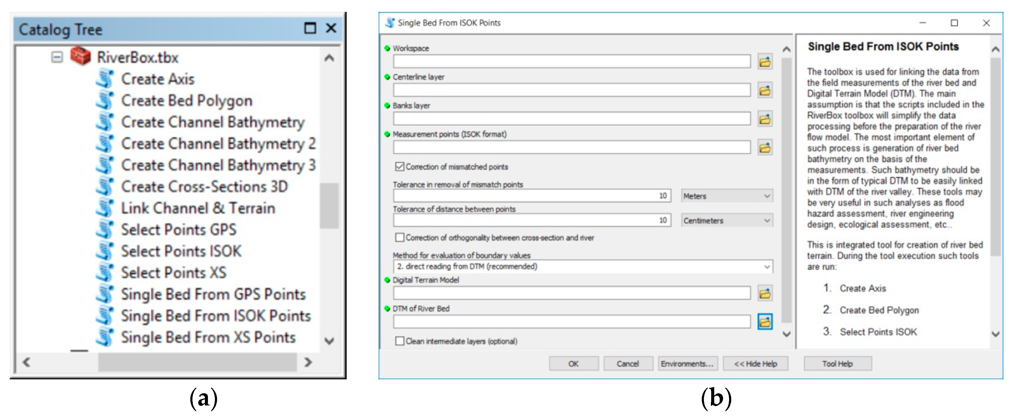
At the current state the developed toolbox called RiverBox is available at the SourceForge web portal. It can be downloaded from https://riverbox.sourceforge.io. The toolbox includes several tools for basic data preparation before interpolation (Figure 7a). These are:
- Create Axis—a tool used for processing of the river centerline and setting linear referencing along it;
- Create Bed Polygon—the tool creates the bed polygon from the bank lines. Such a polygon has linear referencing along its perimeter;
- Select Points ISOK/GPS/XS—three tools applied for selection of points located in the bed polygon. The use of the tool depends on the format of stored points. The formats are described in the Materials section;
- Create Cross-Sections 3D—a tool used for preparation of the 3D lines representing measurement cross-sections.
Other tools are used for bed interpolation. These are
There are also tools integrating the basic steps:
- 8.
- Single Bed From ISOK/GPS/XS points—these tools are prepared for processing the particular format of points and all other necessary procedures. At the present state these tools cooperate only with the first scheme of the bathymetry interpolation.
The last tool is:
- 9.
- Link Channel and Terrain—applied to link the raster of the bed elevations with the basic DEM.
Each tool is prepared using standard methods and GUIs available in ArcGIS (Figure 7b).
There is also basic help attached to each tool and to the majority of the options.
4. Results and Discussion
4.1. Validation Tests of Basic Algorithm
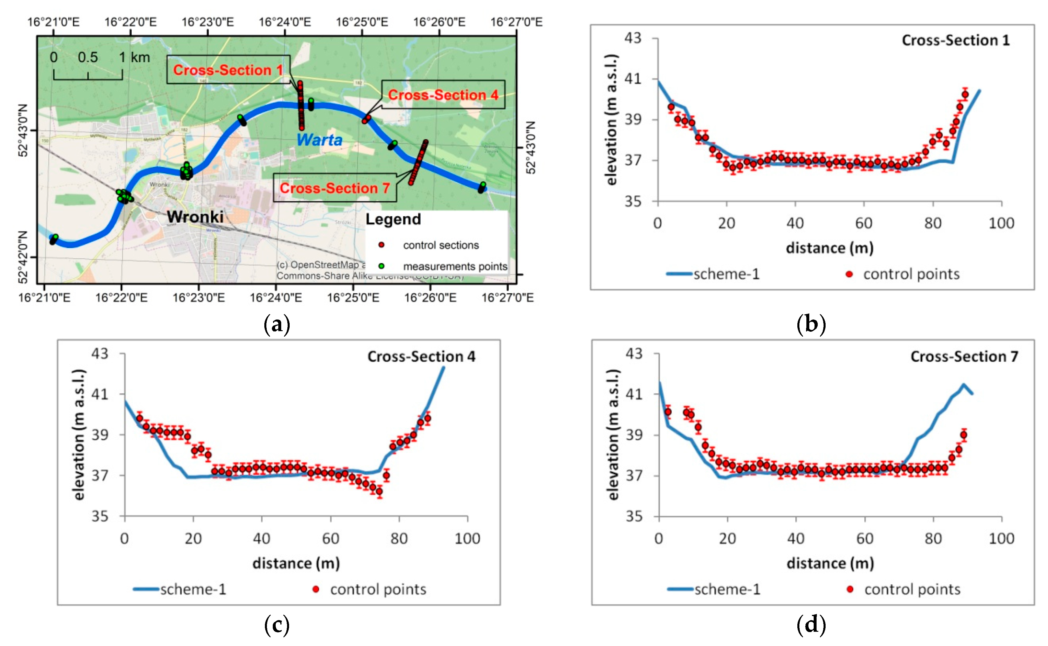
The validation tests are based on comparison of the interpolated bathymetry with measurements taken in 2015, as described in the Materials section. The comparison is done only for the first scheme (Figure 6a), because this scheme is considered to be the reference one. The results of the validation tests are presented in Figure 8. The first element of this composition, Figure 8a, presents the location of cross-sections measured in 2015. They are denoted as cross-section 1, cross-section 4 and cross-section 7. The measured and interpolated cross-section shapes are presented in Figure 8b–d. The blue lines represent the interpolated elevations. The control measurements are presented as red dots with error bars. The error bars equal the previously determined error between measurements and DEM. It is ±31 cm.
Considering comparisons of the validation data with the applied DEM, it is assumed that the interpolated elevation is correct if its value falls into the range determined by error bars. In such a case the error between measurements and interpolation is zero. If the interpolated value is outside of the expected range, then the error is calculated as the difference between the interpolated elevation and the closest value from the desired range. The error statistics are presented in Table 1.
Considering the length of time between the validation data and ISOK measurements, the graph presented in Figure 8b–d shows quite good compatibility between the interpolation and real data. The mean error values presented in Table 1 are 18 cm and 28 cm for cross-sections 1 and 4, respectively. For cross-section 7 this value is 52 cm, but such a high value is caused by the unexplained shift in the cross-section shape. This shift may be caused by some rough errors during measurements or changes in the river morphology in the period 2012–2015.
Hence, the reference interpolation results appear good enough to consider the preparation of the hydrodynamic model for the reconstructed bed.
4.2. Comparison of Tested Algorithms
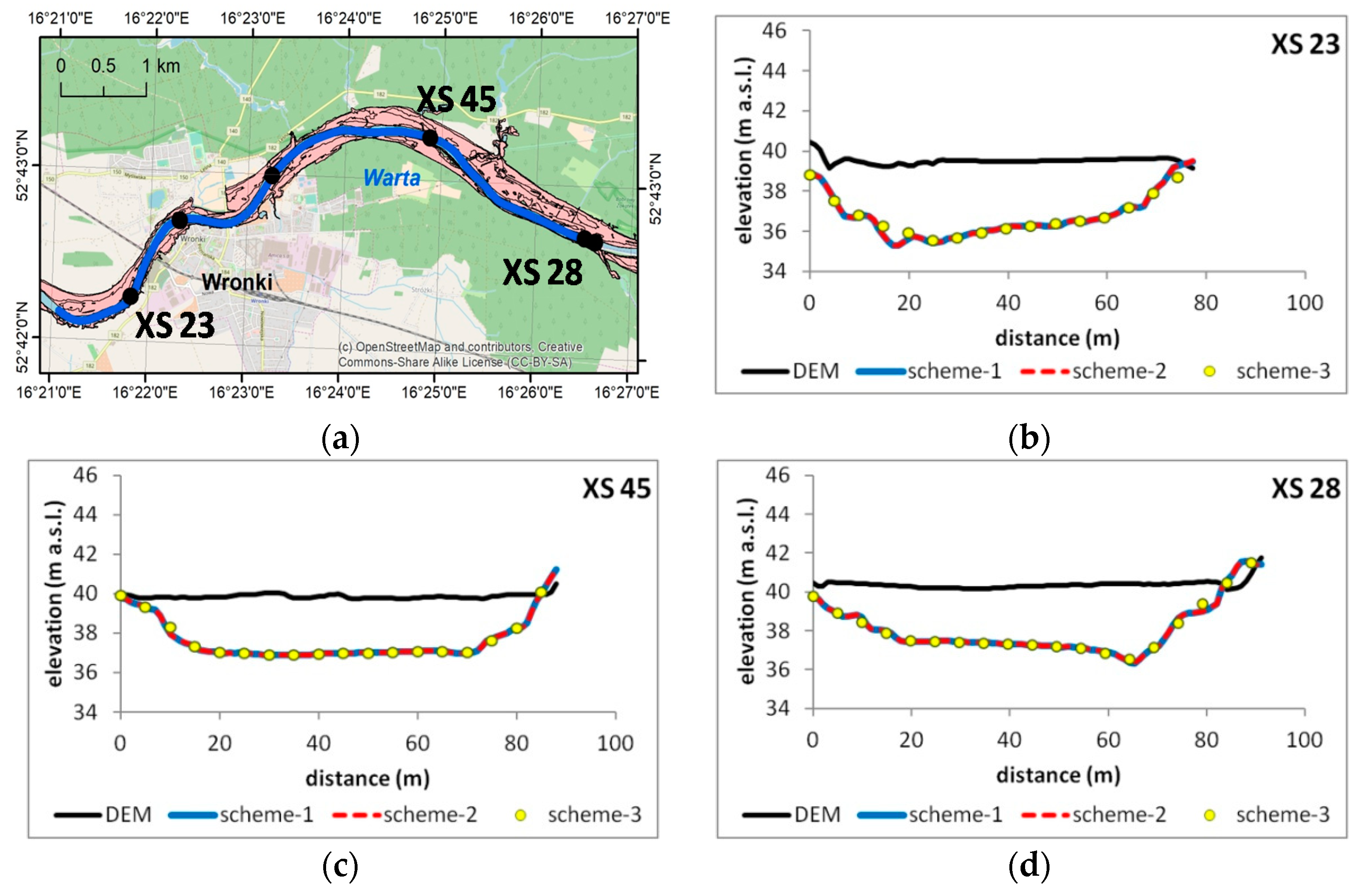
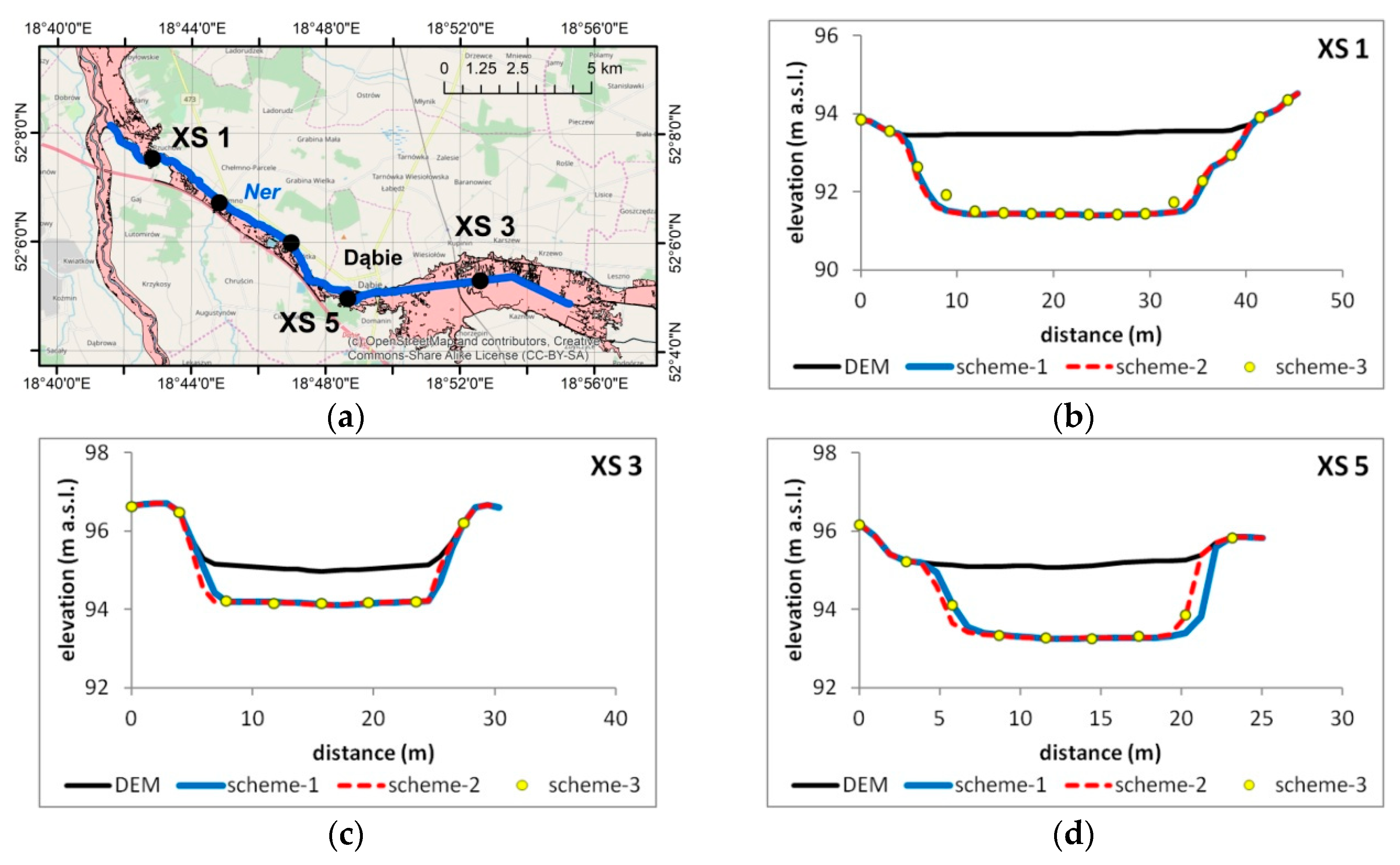
The basic results of the bed interpolation are presented in Figure 9 and Figure 10. The first of them includes results for the first study case—the reach of the Warta river near the town of Wronki. The second presents interpolation of the bed in the Ner river. Each figure includes a map with the location of control cross-sections and graphs of the interpolated cross-section. The background map is the same as that used in Figure 1 and Figure 2. The cross-sections used as examples have labels on the map. Each graph of cross-section shapes includes three lines and one set of points. The black line represents original DEM data. The blue line is obtained as a result of interpolation with the first algorithm based on NumPy arrays (Figure 6a). The red dashed line represents the results of the second algorithm (Figure 6b)—where the points are used instead of NumPy arrays. The last element—the set of yellow points—shows selected results of the third algorithm (Figure 6c) linking longitudinal and spatial interpolations with random points. The last results are obtained for the average density of points reflecting 40 m2 for one point. The measure of density expressed as average area assigned to single points is easier to use than density itself. The boundary points were generated with average density equaling the square root of 40 m2, which is about 6.32 m.
In both cases (Figure 9 and Figure 10) the results are compatible. The second algorithm gives almost the same results as the first one. The results of the third algorithm slightly differ from the previous two, but these differences are not important considering the requirements of the hydrodynamic model geometry. Additionally, the computations of the third algorithm were much faster. For the first case the observed time of computation of the first and the second algorithm was about 30–45 min. The same reconstruction done with the third approach lasted about 4–6 min. In the second case the time of computations was less important than the problems with memory. To apply the first algorithm the whole reach had to be split into two shorter reaches. The second and the third algorithms were able to reconstruct the whole reach at once. Again, the third algorithm was much faster than the first two.
4.3. Efficiency and Accuracy Analysis
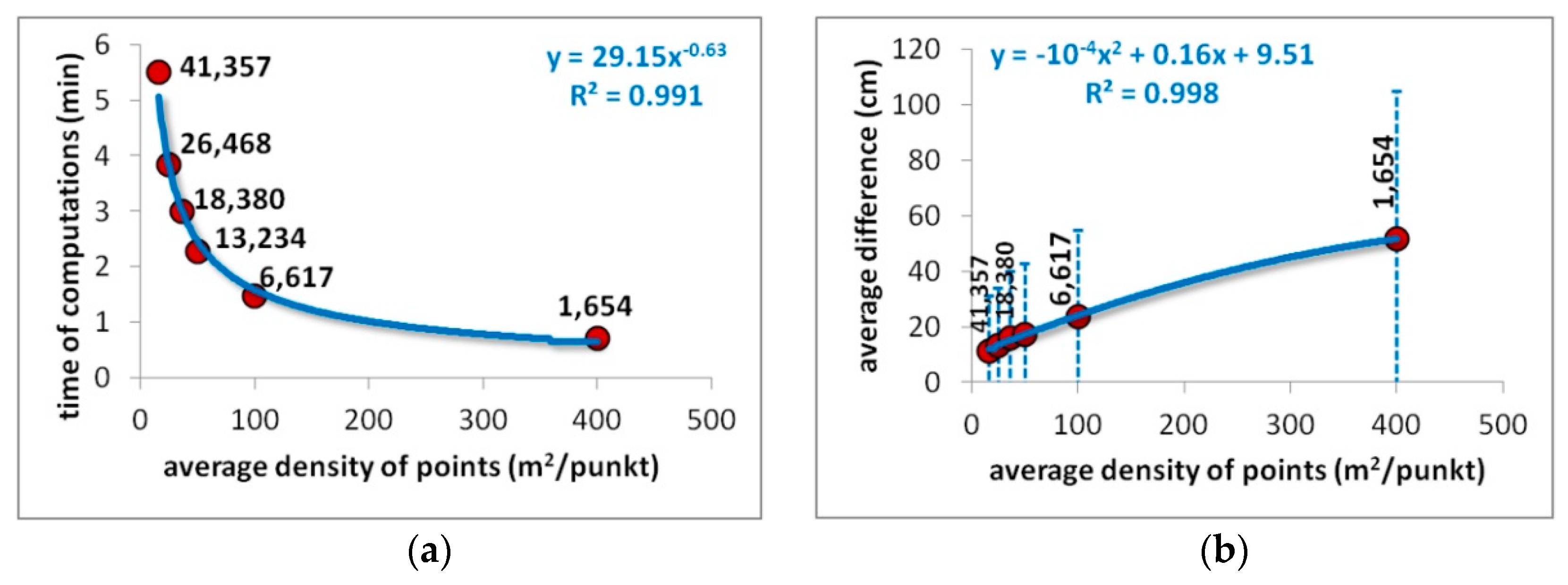
The observed differences in computational time are the inspiration for the next test. Now performance of the third algorithm depending on the average density of generated points is analyzed. As shown previously, the measure of density is expressed as the average area assigned to a single point. The parameters used in these tests are shown in Table 2. The tests were conducted for the first study case, the reach of the Warta river. The average density of points varied from 16 m2 to 400 m2 for one point. The tested densities are listed in third line of Table 2. If the square root of the area is a side of the equivalent square, the average spatial resolution changes from 4 m to 20 m. For the tested case it means that the number of points generated in the bed polygon ranges from 41,357 to 1654, as listed in line 4 of Table 2. Because the third algorithm is random, the reconstruction of the bed bathymetry was calculated 10 times for each density. The computations, for which parameters are shown in the first line of Table 2, were performed on the computer. For each run the time of computations was recorded. Finally, the differences in bed elevations between particular runs and the bed reconstructed with the first algorithm were analyzed at 100 independently generated points (line 6).
The obtained results are presented in Figure 11. The first graph (Figure 11a) presents the dependency of average computational time on the applied average density of points. The time is expressed in minutes. The red dots represent the average computational time for each density. The trend line is used to emphasize the character of this relationship. The second graph (Figure 11b) presents the average differences in elevations in comparison with the results of the first algorithm. These results are overestimated because of the bank points used in the third algorithm which are absent in the other two. However, the graph is used to show the general tendency instead of particular results. As previously, the trend line is used to indicate the kind of dependency analyzed.
In the first graph (Figure 11a) we can see that the acceleration of the computations is proportional to the decrease of the density in the first stage, when the number of points changes from 41,357 to 13,234. In the next stage, with a decrease from 13,234 to 1654, the improvement in computational speed is much smaller. At the same time the dependency of the differences in elevation on the density of points is almost linear. It suggests that there should exist such an optimal point that the acceleration is great, with a relatively small loss of precision in comparison to the first algorithm.
4.4. Discussion
The presented algorithm has several advantages in comparison to the main bed reconstruction tools presented in the scientific papers. As mentioned in the Introduction, the most basic approach was presented by Tate et al. [1]. Such methods are applied in the most popular professional software packages for hydrodynamic simulations, e.g., HEC-RAS and MIKE 11. The drawback of this approach is the lack of channel width information applied during the interpolation process. It may be the reason that the bed contour does not fit the surrounding DEM. This problem is overcome in the presented method. The banks are an important element of the algorithm. The interpolated shape is flexible in the transversal direction due to the application of the relative distance as a coordinate.
The next problem is the comparison of efficiency. In the article by Tate et al. [1] the analysis of computational speed is not presented, though it may not be relevant. Computer processors change very quickly. It was noted that the algorithms implemented in modern hydrodynamic simulation packages are able to interpolate the bed very fast. For example, the interpolation procedure implemented in the HEC-RAS geometry module (Davis, CA, USA), and RAS Mapper (Davis, CA, USA) is very fast. Supposedly, the reason is application of code written in fast Fortran 90/95 and data based on the HDF5 (Hierarchical Data Format 5) format. However, the application of such data requires transformation from typical GIS formats, e.g., GeoTIFF, and back-transformation to GIS formats. Such transformations are also time-consuming. The integration of algorithms with ArcGIS is another advantage of the proposed method.
In studies presented by Merwade and his co-authors [4,5,6,7] the idea of the bed reconstruction is similar, but the implementation is much more complex. The main difference is in the use of an iteratively searched thalweg instead of the arbitrarily chosen centerline. Undoubtedly, the approach with the thalweg is much more time-consuming. As presented in the validation tests, the algorithm with the arbitrary centerline may be accurate enough. The definition of the transversal coordinate as the relative distance from any bank can reduce the problems with arbitrary location of the longitudinal axis. Another difference is the (somewhat complex) determination of the longitudinal and transversal coordinates in Merwade’s studies based on determination of angles. This approach does not protect the algorithm from non-unique zones, such as the no projection and double projection presented in Figure 5b. In the presented algorithm a simpler approach with basic linear projections is implemented. The problem of non-uniqueness is solved with proper correction of the algorithm described in the Methods section.
Other interpolation schemes are presented by Schäppi et al. [13] and Caviedes-Voullième et al. [16]. Both of them are very interesting alternatives to Merwade’s approach if the cross-section measurements are relatively close. In the case of real data scarcity, the scheme proposed by Schäppi and his co-authors may be too weak. The resilience of the second approach described by Caviedes-Voullième and co-authors to this problem is also doubtful. The scheme presented in this paper seems to be more natural, simpler and surely resistant to the problem of sparse data.
5. Conclusions
Today, the technology applied to collect terrain data is based on aerial LIDAR scanning. It is quite a simple method to obtain high-quality data. The resolution of the scanning is appropriate for the majority of applications. Unfortunately, this approach is not able to provide sufficient information about the river and stream bathymetry. This means the DEM created on the basis of the LIDAR scanning does not fit the requirements of hydrodynamic modeling. Additional measurements have to applied. In most cases, GPS technology is used alone or in combination with acoustic or laser scanning of the channel bottom. Such measurements are performed from the ground or from a boat. Because the measurements of the river bed are difficult and time-consuming, the number of such measurements is limited. In most cases the data provided have the form of point-elevation data distributed along selected river cross-sections. The location of the cross-sections is sparse. Finally, the hydrodynamic modeler obtains two sets of data which are not compatible considering the form, resolution, and accuracy. The presented methodology is a way to overcome this problem. The only robust approach is to complete the river bed measurements in such a way that they fit the resolution of the DEM.
In this paper a specific methodology for river bed reconstruction is proposed. It is based on the concept of a channel-oriented coordinate system and basic linear interpolation. Such a simple approach appears to be the best in the case of truly sparse data. The environment chosen for implementation is ArcGIS (version 10.5.1) with the scripting language Python 2.7. The efficiency of the algorithm in the sense of memory usage and computational time is of crucial concern in practical cases. Hence, the ideas presented were implemented in three different computational schemes. The first is based on the raster–array transformation specific to the tools available in the standard Python module attached to ArcGIS and called ArcPy. The results provided are acceptably accurate, as the validation tests show. However, this approach was found to be too slow and with too great memory loading. In the second scheme, the inefficient raster–array transformation is replaced by more robust raster–point transformation. It overcame the problem of memory usage, but the problem of excessive computational time was still important. The main concept of the third scheme is to link two kinds of methods. The first consists of spatial interpolation tools available in the standard Arc Toolbox distributed with ArcGIS. The second is an algorithm developed for bed interpolation in a channel-oriented coordinate system. Such a linkage proved efficient and effective. The loss of potential accuracy is slight, the memory usage is not huge, and the time of computations is much shorter. The third approach is recommended in practical applications.
The algorithm is prepared as a set of tools included in the ArcGIS toolbox called RiverBox. It is open source software. The web address for download is given in the text. The available tools could help in the preparation of the river bed for further hydrodynamic model simulations. Although the toolbox is completed, to properly support preparation of the model for river flow computations further tools have to be added, e.g., interpolation of bed cover information and linking with terrain cover data. An additional problem is transformation of the GIS data to formats valid for hydrodynamic systems, e.g., HEC-RAS, MIKE 11, and others. Such tools will be prepared in the future.
Funding
This research received no external funding.
Acknowledgments
This research would not be possible without the access to the data provided by such institutions as IMGW, CODGiK, GUGiK. The access to the free data available in the Internet such as Geoportal 2 and Open Street Map was also very helpful.
Conflicts of Interest
The author declares no conflict of interest.
References
- Tate, E.C.; Maidment, D.R.; Olivera, F.; Anderson, D.J. Creating a terrain model for floodplain mapping. J. Hydrol. Eng. 2002, 7, 100–108. [Google Scholar] [CrossRef]
- Goff, J.A.; Nordfjord, S. Interpolation of fluvial morphology using channel-oriented coordinate transformation: A case study from the New Jersey shelf. Math. Geol. 2004, 36, 643–658. [Google Scholar] [CrossRef]
- Thompson, J.E.; Warsi, Z.U.A.; Mastin, C.W. Numerical Grid Generation: Foundations and Applications; Elsevier: New York, NY, USA, 1985; Available online: https://web.ics.purdue.edu/~vmerwade/research/terrain_tutorial.pdf (accessed on 7 July 2018).
- Merwade, V.M.; Maidment, D.R.; Hodges, B.R. Geospatial representation of river channels. J. Hydrol. Eng. 2005, 10, 243–251. [Google Scholar] [CrossRef]
- Merwade, V.M.; Maidment, D.R.; Goff, J.A. Anisotropic considerations while interpolating river channel bathymetry. J. Hydrol. 2006, 331, 731–741. [Google Scholar] [CrossRef]
- Merwade, V.; Cook, A.; Coonrod, J. GIS techniques for creating river terrain models for hydrodynamic modeling and flood inundation mapping. Enviro Environ. Model. Softw. 2008, 23, 1300–1311. [Google Scholar] [CrossRef]
- Merwade, V. Effect of spatial trends on interpolation of river bathymetry. J. Hydrol. 2009, 371, 169–181. [Google Scholar] [CrossRef]
- Merwade, V. Creating River Bathymetry Mesh from Cross-Sections; School of Civil Engineering, Purdue University, 2011; Available online: https://web.ics.purdue.edu/~vmerwade/research.html#river (accessed on 7 July 2018).
- Merwade, V. Creating River Bathymetry Mesh from Cross-Sections; School of Civil Engineering, Purdue University, 2014; Available online: https://web.ics.purdue.edu/~vmerwade/research.html#river (accessed on 7 July 2018).
- Merwade, V. Creating River Bathymetry Mesh from Cross-Sections; School of Civil Engineering, Purdue University, 2015; Available online: https://web.ics.purdue.edu/~vmerwade/research.html#river (accessed on 7 July 2018).
- Merwade, V. Creating River Bathymetry Mesh from Cross-Sections; School of Civil Engineering, Purdue University, 2017; Available online: https://web.ics.purdue.edu/~vmerwade/research.html#river (accessed on 7 July 2018).
- Legleiter, C.J.; Kyriakidis, P.C. Forward and inverse transformations between Cartesian and channel-fitted coordinate systems for meandering rivers. Math. Geol. 2007, 38, 927–958. [Google Scholar] [CrossRef]
- Schäppi, B.; Perona, P.; Schneider, P.; Burlando, P. Integrating river cross section measurements with digital terrain models for improved flow modelling applications. Comput. Geosci. 2010, 36, 707–716. [Google Scholar] [CrossRef]
- Bogusz, A.; Orczykowski, T.; Zdralewicz, M. Riverbed interpolation for modeling—Methods comparison. Int. Ecol. Rural Areas 2012, 3, 135–143. (In Polish) [Google Scholar]
- Kardos, M. Interpolating River’s Morphological Model from Cross Sectional Survey. In Proceedings of the Second Conference of Junior Researchers in Civil Engineering; János, J., Róbert, N., Tamás, L., Eds.; Budapest University of Technology & Economics: Budapest, Hungary, 2013; pp. 243–248. [Google Scholar]
- Caviedes-Voullième, D.; Morales-Hernández, M.; López-Marijuan, I.; García-Navarro, P. Reconstruction of 2D river beds by appropriate interpolation of 1D cross-sectional information for flood simulation. Environ. Model. Softw. 2014, 61, 206–228. [Google Scholar] [CrossRef]
- Farina, G.; Alvisi, S.; Franchini, M.; Corato, G.; Moramarco, T. Estimation of bathymetry (and discharge) in natural river cross-sections by using an entropy approach. J. Hydrol. 2015, 527, 20–29. [Google Scholar] [CrossRef]
- Zhang, Y.; Xian, C.; Chen, H.; Grieneisen, M.L.; Liu, J.; Zhang, M. Spatial interpolation of river channel topography using the shortest temporal distance. J. Hydrol. 2016, 542, 450–462. [Google Scholar] [CrossRef]
- Lai, R.; Wang, M.; Yang, M.; Zhang, C. Method based on the Laplace equations to reconstruct the river terrain for two-dimensional hydrodynamic numerical modeling. Comput. Geosci. 2018, 111, 26–38. [Google Scholar] [CrossRef]
- Gnat, R. Reconstruction of Discharge and Water Surface Profile in the Selected Reach of the Ner River. Master’s Thesis, Poznan University of Life Sciences, Poznań, Poland, February 2017. (In Polish). [Google Scholar]
- Press, W.H.; Teukolsky, S.A.; Vetterling, W.T.; Flannery, B.P. Numerical Recipes in Fortran 77. The Art of Scientific Computing, 2nd ed.; Cambridge University Press: Cambridge, UK, 1986; Volume 1, Available online: https://websites.pmc.ucsc.edu/~fnimmo/eart290c_17/NumericalRecipesinF77.pdf (accessed on 7 July 2018).
Figure 1.
Map presenting the first study areas—the reach of the Warta river.

Figure 2.
Map presenting the second study areas—the reach of the Ner river.

Figure 3.
Example of required data: digital elevation model (DEM), polyline layers (river centerline, banks), and measurement points.
Figure 3.
Example of required data: digital elevation model (DEM), polyline layers (river centerline, banks), and measurement points.

Figure 4.
Example of required data: tables of attributes for measurement points.

Figure 5.
Interpretation of basic implemented algorithms: (a) interpolation in channel-oriented coordinates; (b) empty and double projection zones.
Figure 5.
Interpretation of basic implemented algorithms: (a) interpolation in channel-oriented coordinates; (b) empty and double projection zones.

Figure 6.
Tested computational schemes: (a) the first approach based on NumPy array transformation; (b) the second approach based on point–raster transformation; (c) the third approach based on random points.
Figure 6.
Tested computational schemes: (a) the first approach based on NumPy array transformation; (b) the second approach based on point–raster transformation; (c) the third approach based on random points.

Figure 7.
RiverBox presentation: (a) view of the toolbox in the Catalog Tree; (b) example of the tool interface with basic help.
Figure 7.
RiverBox presentation: (a) view of the toolbox in the Catalog Tree; (b) example of the tool interface with basic help.

Figure 8.
Comparison of the bathymetry interpolated with the first algorithm and control cross-sections: (a) location of control cross-sections; (b–d) results of comparison.
Figure 8.
Comparison of the bathymetry interpolated with the first algorithm and control cross-sections: (a) location of control cross-sections; (b–d) results of comparison.

Figure 9.
Comparison of selected cross-sections for the Warta river: (a) Map with locations of the cross-sections used for comparison; (b–d) Compared cross-sections.
Figure 9.
Comparison of selected cross-sections for the Warta river: (a) Map with locations of the cross-sections used for comparison; (b–d) Compared cross-sections.

Figure 10.
Comparison of selected cross-sections for the Ner river: (a) Map with locations of the cross-sections used for comparison; (b–d) compared cross-sections.
Figure 10.
Comparison of selected cross-sections for the Ner river: (a) Map with locations of the cross-sections used for comparison; (b–d) compared cross-sections.

Figure 11.
Results of efficiency tests: (a) Dependency of computational time on density of points in the third algorithm; (b) Dependency of difference between the first and third algorithm on density of points.
Figure 11.
Results of efficiency tests: (a) Dependency of computational time on density of points in the third algorithm; (b) Dependency of difference between the first and third algorithm on density of points.


Table 1.
Error statistics for validation tests.
| Error Statistics (cm) | Cross-Section | ||
|---|---|---|---|
| No.1 | No.4 | No.7 | |
| Max | 123 | 168 | 267 |
| Mean | 18 | 28 | 52 |
| Standard Deviation | 33 | 44 | 83 |
Table 2.
Parameters of efficiency tests.
| Computer | Processor i7-7820HQ, RAM 16 GB, Disk SSD 512 GB | |||||
| Case Study | Warta river near the town of Wronki (7.6 km) | |||||
| Average Density of Points (m2/point) | 16 | 25 | 36 | 50 | 100 | 400 |
| Number of Bed Points | 41,357 | 26,468 | 18,380 | 13,234 | 6617 | 1654 |
| Number of Runs | 10 runs for each density | |||||
| Verification | 100 control points | |||||
© 2018 by the author. Licensee MDPI, Basel, Switzerland. This article is an open access article distributed under the terms and conditions of the Creative Commons Attribution (CC BY) license (http://creativecommons.org/licenses/by/4.0/).
Share and Cite
MDPI and ACS Style
Dysarz, T. Development of RiverBox—An ArcGIS Toolbox for River Bathymetry Reconstruction. Water 2018, 10, 1266. https://doi.org/10.3390/w10091266
AMA Style
Dysarz T. Development of RiverBox—An ArcGIS Toolbox for River Bathymetry Reconstruction. Water. 2018; 10(9):1266. https://doi.org/10.3390/w10091266
Chicago/Turabian StyleDysarz, Tomasz. 2018. "Development of RiverBox—An ArcGIS Toolbox for River Bathymetry Reconstruction" Water 10, no. 9: 1266. https://doi.org/10.3390/w10091266
Note that from the first issue of 2016, this journal uses article numbers instead of page numbers. See further details here.