Irrigation Management Based on Reservoir Operation with an Improved Weed Algorithm

Abstract

Water scarcity is a serious problem throughout the world. One critical part of this problem is supplying sufficient water to meet irrigation demands for agricultural production. The present study introduced an improved weed algorithm for reservoir operation with the aim of decreasing irrigation deficits. The Aswan High Dam, one of the most important dams in Egypt, was selected for this study to supply irrigation demands. The improved weed algorithm (IWA) had developed local search ability so that the exploration ability for the IWA increased and it could escape from local optima. Three inflows (low, medium and high) to the reservoir were considered for the downstream demands. For example, the average solution for the IWA at high inflow was 0.985 while it was 1.037, 1.040, 1.115 and 1.121 for the weed algorithm (WA), bat algorithm (BA), improved particle swarm optimization algorithm (IPSOA) and genetic algorithm (GA). This meant that the IWA decreased the objective function for high inflow by 5.01%, 5.20%, 11.65% and 12% compared to the WA, BA, IPSOA and GA, respectively. The computational time for the IWA at high inflow was 22 s, which was 12%, 18%, 24% and 29% lower than the WA, BA, IPSOA and GA, respectively. Results indicated that the IWA could meet the demands at all three inflows. The reliability index for the IWA for the three inflows was greater than the WA, BA, IPSOA and GA, meaning that the released water based on IWA could well supply the downstream demands. Thus, the improved weed algorithm is suggested for solving complex problems in water resources management.

1. Introduction

Water resources management is an important area of hydrological sciences that deals with the sustainable allocation and utilization of water as a valuable resource [1]. Water scarcity has been identified as a major problem for water resource managers in different regions throughout the world. Technologies and innovative ideas need to be explored and embraced to resolve this practical challenge through strategic decisions made about water utilization [2,3]. Optimizing reservoir operation is one of the most important approaches to solving water scarcity. In this regard, a suitable optimization algorithm that allows core decision-markers to generate optimal operating rules for water utilization and to minimize perceived gaps between water release and demand is practical for water resources management [4]. A primary aim for controlling a reservoir’s operation is to develop a set of rules that govern the controlled release of water for downstream users that lead to a reduction in water shortages [5]. It is also imperative to ensure that the amount of water stored in the reservoir is not less than the permissible range used in the dry season and during critical conditions [6]. Consequently, new measures implemented for the controlled release of water and to provide a sustainable water supply to the different water users (e.g., those engaged in industrial activities and in agricultural practices), must be identified through an appropriately selected optimization algorithm to resolve the issues faced in the operation of a reservoir [7,8].

Over the last two decades, evolutionary and meta-heuristic optimization methods have been developed and explored to solve complex engineering-based optimization problems. A major advantage of these approaches lies is their simplicity for adjusting the objective function and the system constraints within the method’s mathematical process. On the other hand, attaining the global optima that allow a universal solution can be a time-consuming process and thus, it is undesirable for real-time operation purposes. It has been shown that evolutionary and meta-heuristic methods involve less computational time in solving a complex problem and therefore may be useful for core decision-makers who need to attain an optimal solution for real-time problem-solving [4].

1.1. Background

Fallah Mehdipour et al. [9] applied genetic programming for reservoir operation to reduce irrigation deficits. The released water for downstream was considered as decision variables and different arithmetic and mathematical operators were tested for the genetic programming. The results indicated that the irrigation demands were met with the highest reliability index compared to the genetic algorithm (GA) and particle swarm optimization (PSO). The decision variable for the study was the released water as an unknown value.

Ostadrahimi et al. [10] applied PSO for multi-reservoir operation to generate different rule curves to reduce irrigation deficits for a case study in Iran. The applied PSO acted based on modified inertia weight as new version of PSO algorithm to increase the convergence rate. The results were compared with the GA and nonlinear programming. The PSO had greater convergence velocity than the GA and based on PSO, the released water could meet irrigation demands.

Afsahr [5] optimized reservoir operation with a modified and adapted version of PSO with the aim of increasing the benefits of power generation. This version of PSO adapted with the hydrological and hydraulic boundary condition of problem so that the algorithm could model the reservoir operation during the drought years. The new version of PSO had average solutions that were close to the global solution of the problem and annual generated power was greater than that calculated by the GA and harmony search algorithm (HA).

Ant colony optimization (ACO) was used for the optimal operation of multi-reservoir systems and results indicated that the applied algorithm could meet irrigation demands with the least risk so that the average irrigation deficit was reduced to a probable minimum value [11]. Also, Moeini and Afshar [11] developed the ACO based on mutation operator to increase the diversity for the initial population of algorithm.

Zhang et al. [12] applied a new dynamic programming method and GA for the operation of a multi-reservoir system with the aim of increasing of power generation in the China. The GA had a better performance than dynamic programming although the power generation for the dry years accorded with the limitation so that a rationing process could be good strategy for dry years.

The water cycle algorithm (WCA) was used for reducing power deficits based on the movement of drops in the environment and with the positions of drops considered as the initial population [13]. The position of drops in the environment was considered as a decision variable and the algorithm acted based on movement of drops to the rivers. The computational time of the WCA was decreased compared to the GA and PSO and the averages of deficits were decreased by the WCA to the probable minimum value.

Bozorg-Hadad et al. [14] applied the bat algorithm (BA) with the aim of decreasing of power deficits for a case study in Iran. The algorithm is based on the received frequencies of bats from their surroundings. The position of bats were considered as decision variables and they were updated based on velocity and frequency value. The convergence velocity for the BA based on a random walk and local search process was more than the GA and PSO and the BA power generation process had a higher reliability index.

Different orders of nonlinear rule curves based on the GA were used for the operation of a reservoir [15]. Results indicated that the third order rule curve could meet irrigation demand based on the high value obtained for the reliability index so that the released water met demands well and irrigation deficits were minimized.

Biogeography based optimization (BBO) was used for decreasing power deficits for a case study in Iran [16]. The algorithm was based on environmental habitats and migration processes in the environment. Results indicated that the algorithm could generate solutions which were close to the global solution based on less iteration. The process of the algorithm was simple and based on an initial population of species in the environment.

Asghari et al. [17] applied the weed optimization algorithm (WA), based on weeds growing in the environment, for multi-reservoir operation with the aim of increasing power generation. The results were compared with the GA, PSO and WCA and indicated that the WA had the greatest convergence rate and highest values of the generated benefits.

Fixed length genetic programming (FLGP) was used for the operation of a multi-reservoir system with the aim of decreasing irrigation demands [18]. Results indicated that the demand for irrigation could be supplied based on FLGP, which had a higher reliability index than GP and a greater convergence velocity than other algorithms.

The gravity search (GS) algorithm was used for a multi-reservoir system with the aim of decreasing power generation [19]. The results indicated that the GS needs to the accurate sensitivity analysis for the random parameters in the algorithm. Annual power generation based on GS had a higher value and greater convergence velocity than the GA and PSO.

The shark algorithm (SA) based on shark life and rotational movement was applied to reservoir operation to reduce irrigation deficits [20]. The rotational movement was considered as having powerful ability to avoid trapping in the local optimums. Results indicated that the SA could supply the irrigation demands based on a higher reliability index compared to the PSO and GA. The SA also had a greater convergence speed than the GA and PSO.

Ehteram et al. [21] applied monarch butterfly optimization algorithm for the multi reservoir systems in the China. The algorithm acted based on migration operator for the butterflies. The results indicated that the annual average for power production based on monarch algorithm was 12% and 14% more than GA and PSO.

Mousavi et al. [22] applied the crow algorithm for the extraction of rule curves for the irrigation management for a case study. The algorithm acted based on ability of crows for the finding and hiding of food. The results indicated that the vulnerability index based on crow algorithm was decreased significantly by the crow algorithm.

Karami et al. [23] applied the krill algorithm for reservoir operation and irrigation management. The initial position of krill was considered as decision variable and the results indicated the average annual for irrigation deficits based on krill algorithm was 20% and 23% less than PSO and genetic algorithm.

The kidney algorithm (KA), based on the way a kidney performs in the body, was used for the operation of a reservoir with the aim of decreasing power generation [24]. The KA had a simpler optimization process than the GA, PSO and HA and the vulnerability index for power generation was decreased 10%, 12% and 14% by KA compared to the PSO, HA and GA, respectively.

Ehteram et al. [25] applied the spider monkey algorithm based on monkey life. The local and global leaders were considered as important future of these algorithms and the method was used for irrigation management for multi reservoir in Iran. The results indicated that spider monkey algorithm could the downstream demands based on higher reliability index compared to the genetic algorithm and particle swarm algorithm.

Karami et al. [26] applied the simple weed algorithm for irrigation management for a case study in Iran. The results indicated that the annual average of deficits based on WA was more than PSO and the algorithm did not have the good convergence velocity.

1.2. Innovation and Objectives

One of the known algorithms in the field of optimization is the weed algorithm (WA). This algorithm acts based on weed life and the processes of generating weeds and seeds in the environment. One of the main advantages of the WA is related to its simple architecture in the optimization process and the simple method of setting the random parameters. The WA has been used in different fields such as training controller robots [27], designing recommender systems [28], optimization of mathematical benchmarks [29], optimization of power plant performance [23] and optimization of reservoir performance [17]. Asghari et al. [17] applied the weed algorithm for reservoir operation based on increasing of power generation for downstream power plant. The results indicated that the weed algorithm needed to high computational time compared to the PSO. Karami et al. [23] applied the weed algorithm for the decreasing of irrigation deficits and the results indicated the annual average deficits for the WA was 20% PSO and also, the algorithm could not obtain the global solution for the benchmark with some local optimums.

One of the main weaknesses of the WA is a tendency to get trapped in local optima. Another challenge is related to the exploration ability, which allows the algorithm to search a large volume in the problem space and find the best solution (close to the global solution) in the least computational time [17]. Thus, it is necessary that the WA be improved based on new operators in the local search section of algorithm. The new algorithm is defined in this study based on an elite weed. One level and an operator are added to the algorithm to search the space around the elite weed within a specific radius [23]. This ability causes new weeds to be generated during the WA optimization so that the algorithm can exit from the local optima and the diversity of population is added with the improved WA (IWA). The increased population diversity and the improved ability of the WA search, results in better potential for finding the best solution based on a more accurate search around of global solution. Thus, the paper address these issues: (1) prepare improved weed algorithm based on new operators, (2) formulate the mathematical weed algorithm for the reservoir operation, (3) introduce comprehensive study based on comparing of new weed algorithm with other evolutionary algorithms, (4) examine the new weed algorithm based on different inflows to the reservoir with the aim of irrigation deficits. In fact, the IWA has more ability to avoid trapping in local optimum and experienced less computational time compared to the classical WA. These two advantages provide the IWA the ability to search for the global optima and better suitability over the other algorithms to be proposed for real-time application. In addition, the IWA has experienced good balance between exploration and exploitation ability.

The Aswan High Dam in Egypt, an important dam for increasing water storage for irrigation demand in areas downstream of the dam, is used as a case study. This dam plays an important role in Egyptian economics. Reports showed that the monetary benefit generated after dam construction was 255 million USD of which 180 USD was related to agricultural production and indicates the importance of the Aswan High Dam for meeting irrigation demands. In our study, the IWA is used for optimal operation of this dam with the aim of reducing irrigation deficits and results are compared with the weed algorithm (WA), bat algorithm (BA), improved particle swarm optimization algorithm (IPSOA) and the genetic algorithm (GA). The reliability index, vulnerability index and resiliency index are used to evaluate the new weed algorithm relative to the other evolutionary algorithms for its performance in meeting irrigation demands. The output of this paper will show the amount of water storage required at different inflows to meet water demands of the IWA compared to the other algorithms for this important problem in water resources management. The main innovation of this paper is related to the improvement of the WA and its application in water resources management.

2. Method

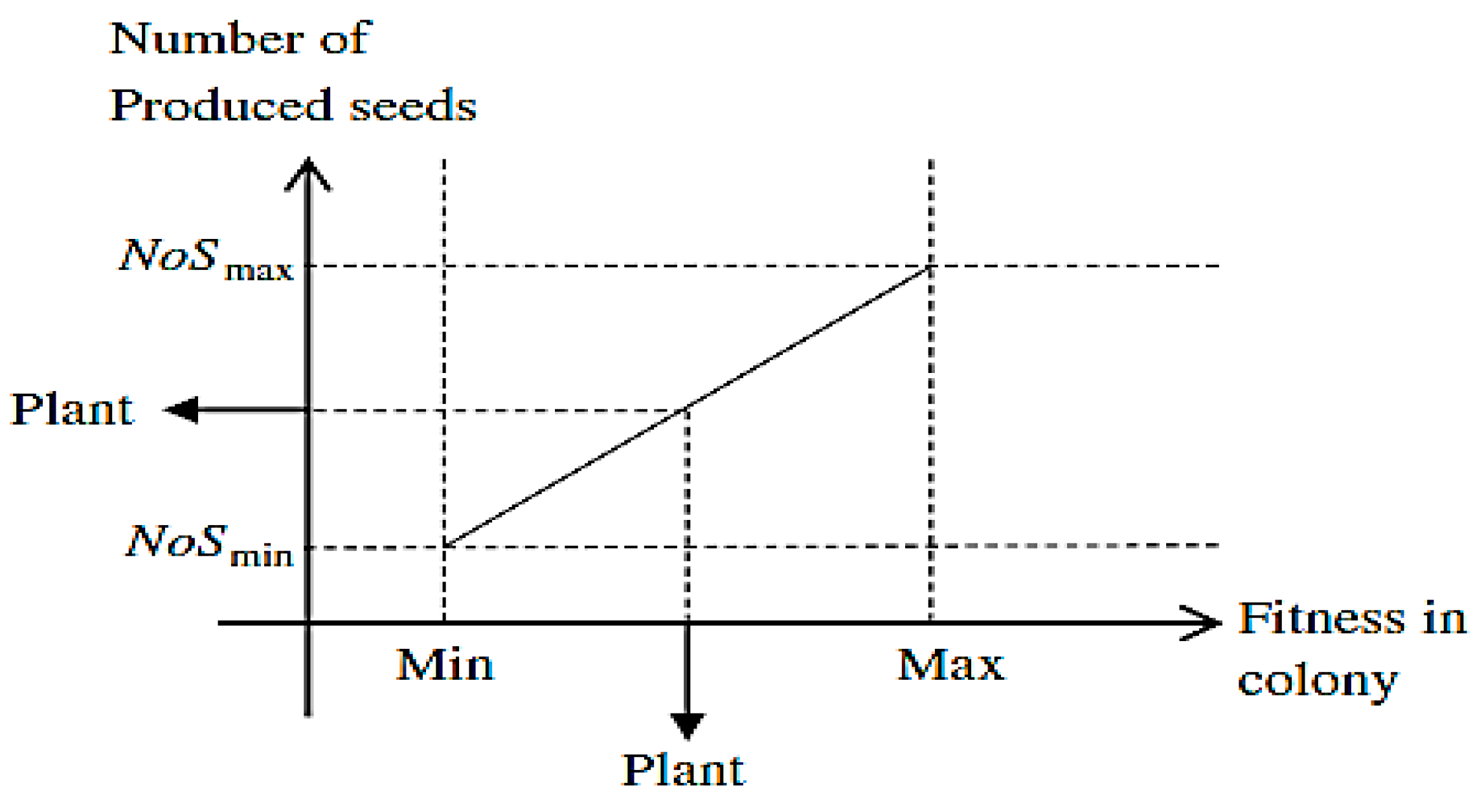
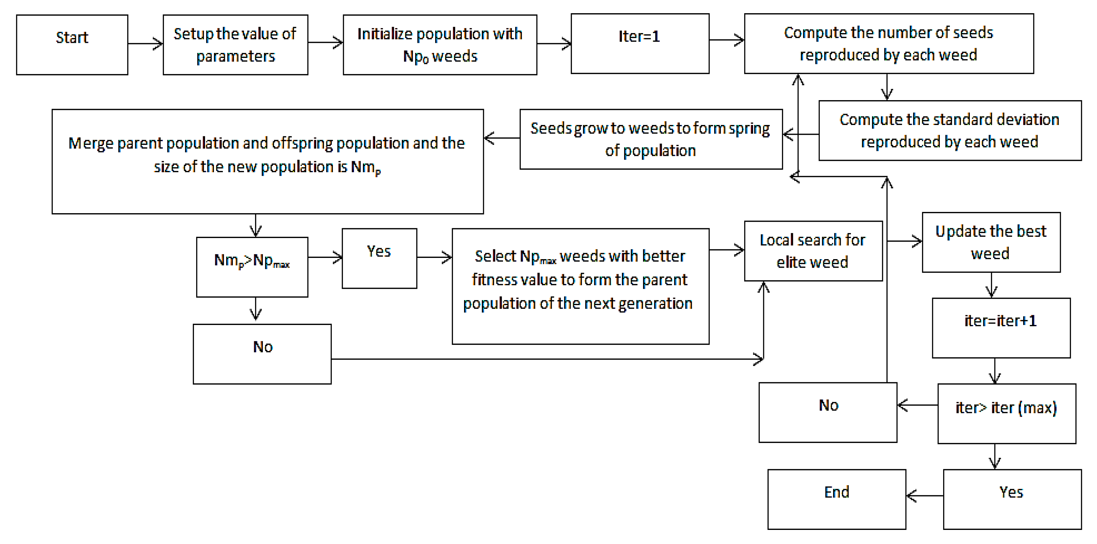
2.1. Weed Algorithm (WA)

The WA acts based on weed behavior in the environment and each weed is considered one solution. The initial weed population for the algorithm is NP₀. The weeds produce seeds with a normal distribution and these seeds can grow and become offspring weeds; the offspring weeds and the parent weeds generate the next population for the WA. The weed with the best value for the objective function is selected and the iteration cycle continues until the convergence criteria are satisfied. The following assumptions are considered for the algorithm [17]:

• A limited number of seeds can grow in the environment.
• The seeds can grow and become weeds to continue the next generation.
• The growth process and generation of seeds and weeds continue until the number of seeds reaches a maximum number.
  The algorithm is considered based on the following levels:

2.1.1. Initialization

The size of the initial population equals NP₀. Each weed is considered as a solution candidate so that the accurate size of the population and the value of NP₀ are determined based on sensitivity analysis.

2.1.2. Reproduction

Reproduction is a process where the weeds generate seeds and the maximum and minimum number of seeds, N₀S_max and NS_min, are generated based on the quality of parent weeds. Weeds that live in one location are known as a colony [17]. Reproduction is important because although plants of lower quality have a smaller chance of continuing of their presence in the next generation, the process allows even the low-quality plants (weeds) to generate seeds because they may contain important information. Figure 1 shows the production level of the WA.

The number of generated seeds is computed based on the equation

$$Nsee{d}_j=N{S}_{min}+\frac{Fi{t}_j-Fi{t}_{min}}{Fi{t}_{max}-Fi{t}_{min}}\times \left(N{S}_{max}-N{S}_{min}\right)$$

(1)

where, $Fi{t}_j$ is the jth objective function, $Fi{t}_{min}$ is the minimum value of the objective function, $Fi{t}_{max}$ is the maximum value of the objective function and $Nsee{d}_j$ is the number of seeds in each level.

2.1.3. Spatial Dispersal

The seeds generated by weeds are distributed randomly. The generated offspring weeds are distributed according to a mean 0 and a standard deviation. The standard deviation is considered a large positive value and it decreases as the number of iterations increases. This results in the combination of the global search and local search to get the optimal search space. The standard deviation is computed based on the equation

$${\sigma }_{iter}=\frac{{\left(I{t}_{max}-Iter\right)}^t}{I{t}_{max}}\times {\left({\sigma }_{initial}-{\sigma }_{final}\right)}^2+{\sigma }_{final}$$

(2)

where ${\sigma }_{iter}$ is the standard deviation for each level, $I{t}_{max}$ is the maximum number of iterations, $Iter$ is the number of iterations in each level, ${\sigma }_{initial}$ is the initial standard deviation, ${\sigma }_{final}$ is the final standard deviation and t is the nonlinear modulus

2.1.4. Competitive Selection

Weeds do not go extinct as long as they can generate offspring weeds. There is a limit to the number of weeds that could live in the environment. When the weeds generate offspring weeds, they constitute the next generation for the population. If their number is not more than NP₀, there is not a specific problem; otherwise, the NP₀ weed with the better objective function based on a competition is selected for continuing the algorithm. The weed with the best value for the objective function is then selected in the new population; if it is better than the best weed computed so far, the new weed will replace the previous best weed.

2.2. Improved Weed Algorithm (IWA)

Local search ability is added to the WA to increase the searches of the problem space and give the algorithm more exploration ability to obtain optimal solutions. First, the weed with the best value for the objective function is selected as the elite weed. N_es seeds are then produced by the elite weed. The new seeds grow around the elite weed and generate new weeds, which grow within a radius S_r from the elite weed. Each new weed, as one of the decision variables, can be defined based on

$$x_{\left(new\right)s,i}=x_{s,i}.\left(rand\left(\right)\times 2\times S_r+\left(1-S_r\right)\right)$$

(3)

where $x_{\left(new\right)s,i}$ is the new value of the weed for the ith variable, $x_{s,i}$ is the value of ith weed and $S_r$ is the radius.

Then, the computed value for the weeds is checked with the upper and lower values of the decision variables

$$x_{s,i}=\left[\begin{array}{l}{x}_{min}\leftarrow if\left(x_{s,i}\right)<x_{min}\\ x_{max}\leftarrow if\left(x_{s,i}\right)>x_{max}\end{array}\right]$$

(4)

where $x_{min}$ is the lower limit for the decision variable and $x_{max}$ is the upper limit for the decision variable.

Figure 2 shows the IWA process.

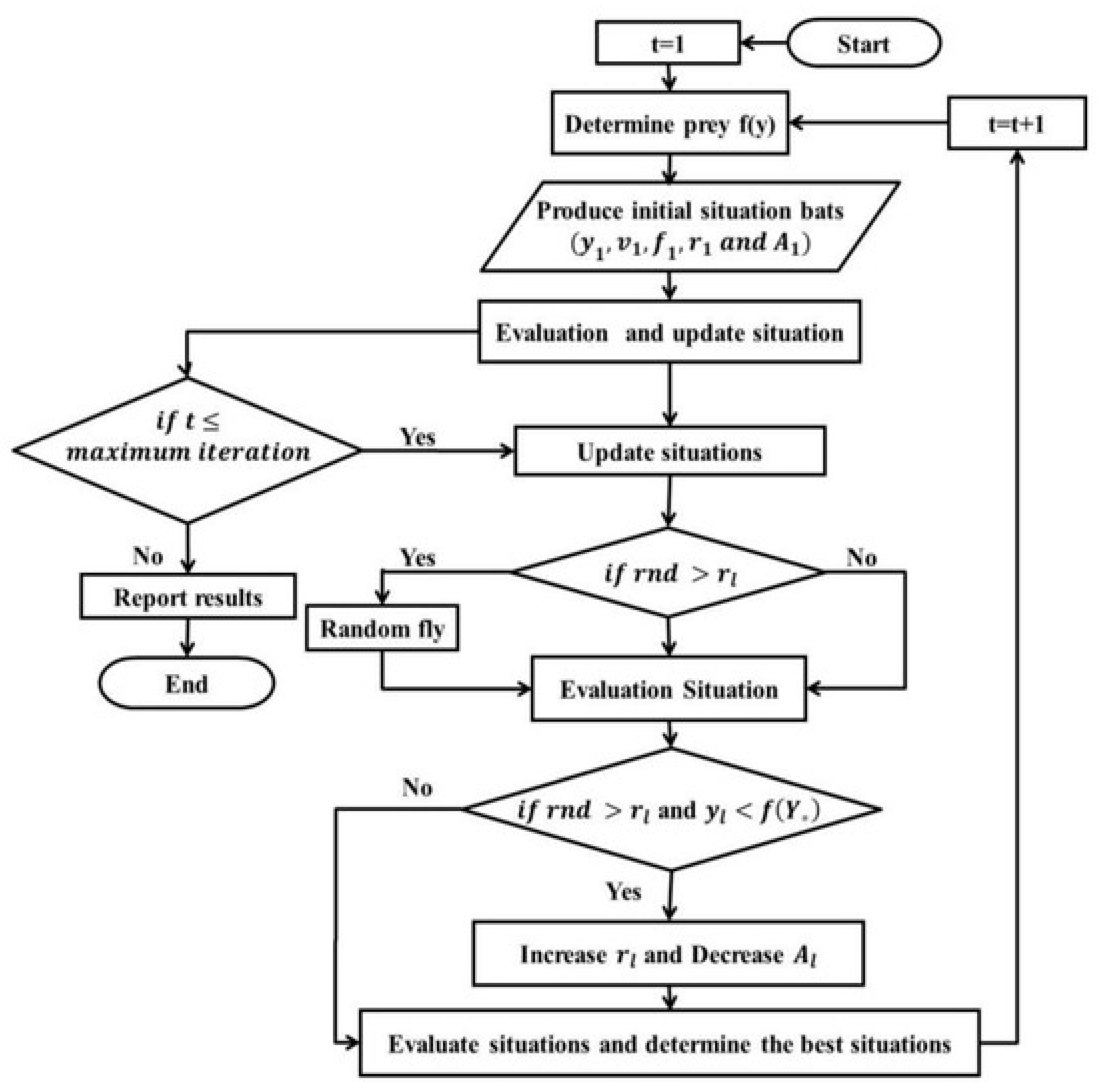
2.3. Bat Algorithm (BA)

Bats have a powerful ability to receive sounds from their surroundings. They generate sounds, which are echoed back and allow the bats to distinguish obstacles from food based on the received frequencies. The BA acts based on the following assumptions [21]:

• The echolocation ability is used by all bats so that they can identify an obstacle in their surroundings.
• Bats have random velocity ($v_l$) at a random position (y_l) and the frequency, wavelength and loudness for the BA are $f_l$, $\lambda$ and A, respectively.
• The loudness varies for the bats from a large positive to a small positive.

The sounds generated by the bats have a pulsation rate (r_l), which is between 0 (minimum) and 1 (maximum). The position, pulsation rate and frequency are updated based on the equations

$$f_l=f_{\min }+\left(f_{\max }-f_{\min }\right)\times \beta$$

(5)

$$v_l\left(t\right)=\left[y_l\left(t\right)-Y_{\ast }\right]\times f_l$$

(6)

$$y_l\left(t\right)=y_l\left(t-1\right)+v_l\left(t\right)\times t$$

(7)

where $f_{min}$ is the minimum, $f_{max}$ is the maximum frequency, $Y_{\ast }$ is the best solution, $v_l\left(t\right)$ is the velocity, t is time interval, $y_l\left(t-1\right)$ is position at time (t − 1), $\beta$ is the random vector and $f_l$ is the frequency.

The random walk is used as a local search strategy

$$y\left(t\right)=y\left(t-1\right)+\epsilon A\left(t\right)$$

(8)

where $\epsilon$ is a random value between −1 and 1 and $A\left(t\right)$ is loudness.

The loudness and pulsation rate are updated for each level. When the bats find prey, the pulsation rate increases and the loudness decreases and also, there is this condition vice versa. The pulsation rate is updated based on

$$r_l^{t+1}=r_l^0\left[1-\exp \left(-\gamma t\right)\right]A_l^{t+1}=\alpha A_l^t$$

(9)

where $\alpha$ and $\gamma$ are constant parameters. The BA process is shown in Figure 3.

2.4. Improved Particle Swarm Optimization Algorithm (IPSOA)

The optimization process in this algorithm starts with the collection of particles. Each particle is considered as a candidate solution of the optimization problem and contains three vectors: the current position of the particle (x_i), the best-obtained position of each particle in the previous iteration (y_i) and the velocity vector. A central aim of each cycle in the algorithm is the identification of the best position of each particle [18]. Following this, the best position of the particle (X_i^iter+1) is considered as the new position of the new particle for the purpose of continuance in such a way that it yields two main equations [23]

$$V_i^{iter+1}=w{V}_i^{iter}+c_{1}rnd\left(Y_i^{iter}-X_i^{iter}\right)+c_{2}rnd\left(Y_{*}^{iter}-X_i^{iter}\right)$$

(10)

$$X_i^{iter+1}=X_i^{iter}+V_i^{iter+1}$$

(11)

where $V_i^{iter+1}$ is the new velocity vector for each particle, c₁ is the personal learning coefficient, $c_2$ is the global learning coefficient, rnd is a random value between 0 and 1, $Y_{*}^{iter}$ is the current best solution and w is the inertial coefficient.

Past experimental results have shown that it is better to consider high values for the inertia coefficient at the start of the process because the algorithm is able to search the solution space with a higher accuracy and its value can be reduced linearly. In this study, an improved version of the PSOA (denoted as IPSOA) was used for solving the optimization problem where the following equation shows the linear reduction in the inertial coefficient

$$w^{iter+1}=w^{iter}\times w_{damp}$$

(12)

where w_damp is a reduction (damping) coefficient bounded by (0.9–1).

In order to optimize the given problem, the particles in the algorithm spread in the search space and they are improved by the best solutions, which are found in each iteration of the search space. The second term in Equation (10) is the internal knowledge of each particle, which compares its current position to the previous best position. The third term in this equation shows the social interaction among the particles, which is used to measure the difference between the current and the best position of each particle.

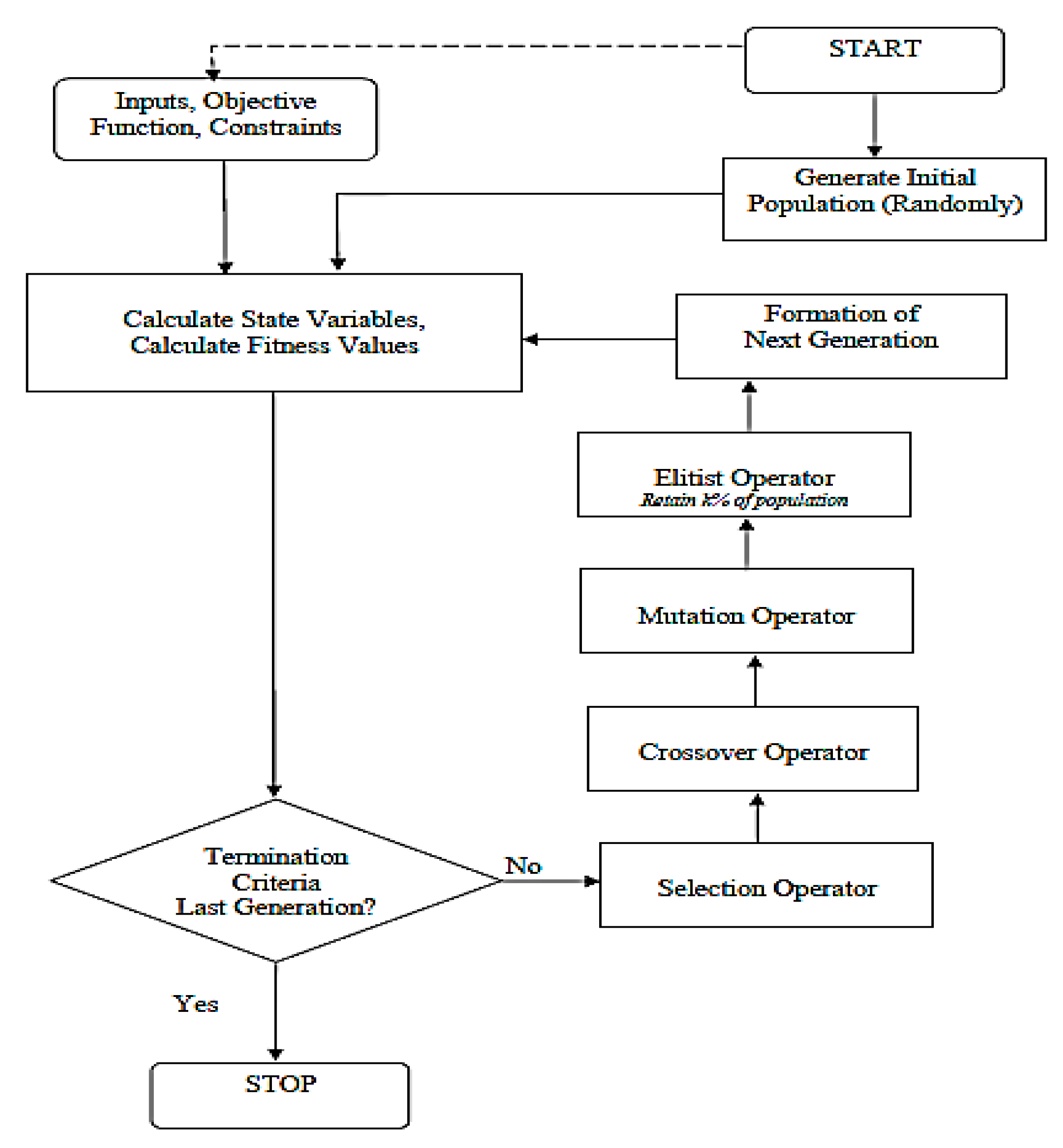
2.5. Genetic Algorithm (GA)

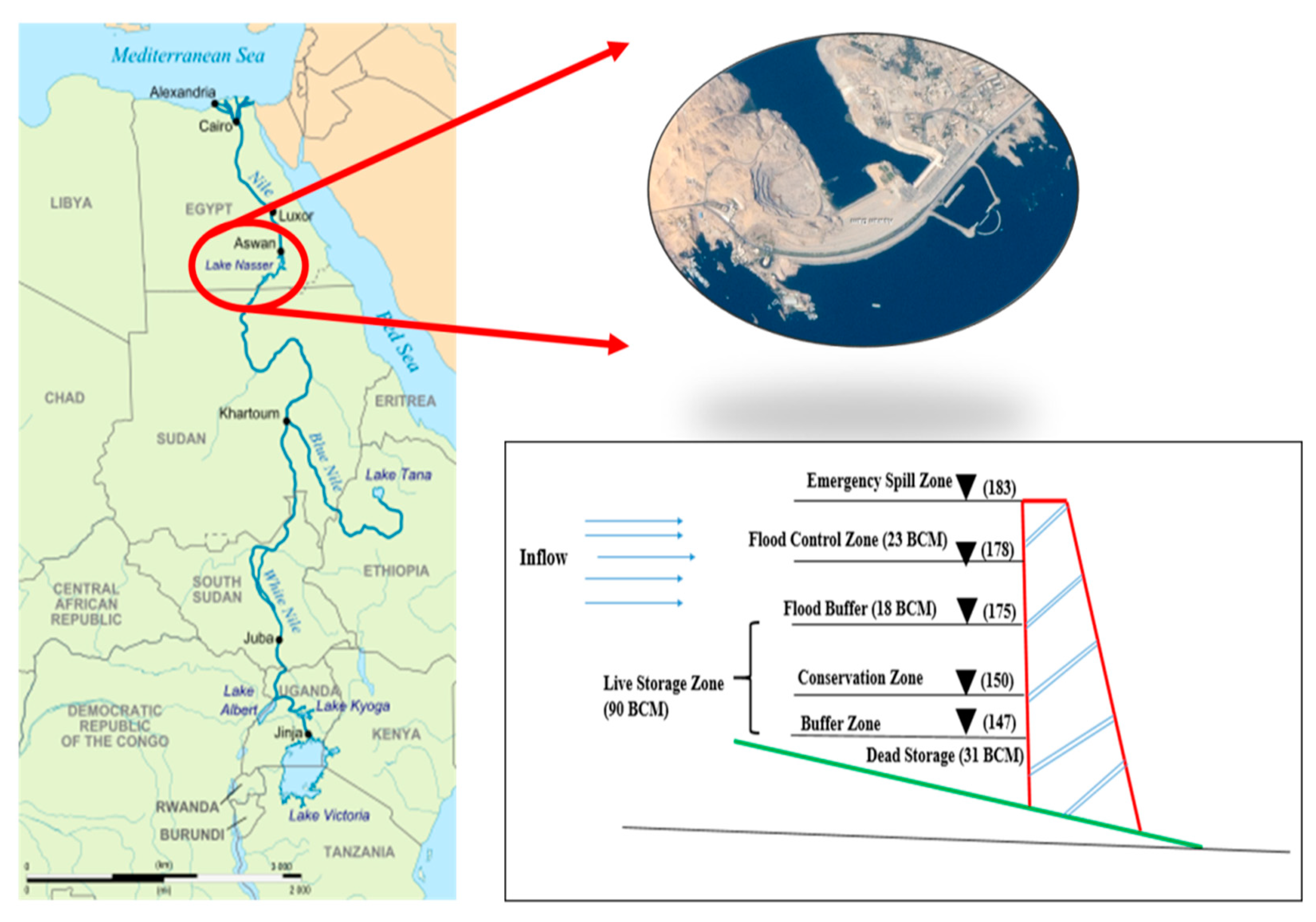
Decision variables in the GA are defined based on a random population and its chromosomes. A particular code is considered for each variable and the fitness function is then computed based on the initial value of each chromosome assigned to the problem of interest [23]. Each chromosome has an objective function and the operator selection chooses the best chromosome. These superior chromosomes are considered for crossover operators to generate new chromosomes based on the parents’ characteristics. Following this, the mutation operator is used for the change of one or more genes for the generation of better chromosomes. Figure 4 shows the schematic diagram of the GA.

3. Case Study

The case study site, Aswan High Dam (AHD), located on the Nile River, is the highest dam in Egypt (Figure 5).

Minimizing the water deficit downstream from the dam is considered as an objective function in terms of the optimization problem that needs to be solved for core decision-making and for optimal water resources management. The AHD is one of the largest dams in the world and has a relatively large reservoir, namely Lake Nasser that lies between latitudes 22°00″ and 23°58″ N and longitudes of 31°07″ and 33°15″ E. Lake Nasser has a maximum width of 60 km and a mean width of 10 km. Data of monthly inflow to the reservoir is extracted from 1989 to 1999 because there is a real water scarce for this period. Inflow is classified based on the United State Geological Survey (USGS). A value on a scale of 100, known as a percentile, indicates inflow distribution. For example, when river discharge on a specific day is in the 70th percentile, it means that this discharge is equal to or greater than 70% of discharge recorded on this day of the year during all years that measurements have been made. The USGS suggests that a percentile of more than 75 is high inflow and a percentile below 25 is low inflow. Normal inflow means the percentile is between 25 to 75.

Table 1. Classification of monthly inflow to the reservoir (BCM) (1989–1999).

Month	High	Medium	Low	Demand
	Billion Cubic Meters (BCM)
January	4.8	3.15	1.90	3.5
February	3.7	1.95	0.80	3.8
March	3.5	1.7	0.55	4.4
April	2.7	1.15	0.30	4.9
May	2.5	1.35	0.65	5.1
June	2.8	1.65	0.90	5.2
July	7.7	4.75	2.80	5.8
August	27.5	20.4	15.50	5.1
September	31	24.05	18.55	4.5
October	21.2	15.6	11.3	3.9
November	10.9	7.30	4.75	3.2
December	6.5	4.30	2.7	2.9

shows the classification of average monthly inflows into the reservoir during 1989 to 1999.

Several parameters of the AHD reservoir were limited to satisfy the optimization model. Eleven values were considered for the initial reservoir storage and the model was then executed for each storage value and three inflow scenarios (i.e., high, medium and low). This yielded a total of 36 rule curves for a one-year period. The required information was extracted from the study of El-Shafie et al. [30] where the seepage value for the reservoir was set at 0.08 billion cubic meters (BCM) and the water level was to be maintained over the range 147–183 m. The permissible range in storage was approximately 32–162 BCM and the maximum value for water release was approximately 7.5 BCM. For this dam, the water level at the end of July was expected to be less than 175 m (122 BCM). The objective function for this reservoir is

$$\min imizeZ={{\displaystyle \sum _{t=1}^1\left(D_t-R_t\right)}}^2$$

(13)

where Z is the objective function, D_t is the water demand (BCM) and R_t is the water release (BCM).

The constraints for this problem are explained in the following equations.

Continuity equation:

$$S_{t+1}=S_t+I_t-R_t-L_t$$

(14)

where S_t+1 is the storage at the end of the period t, S_t is the storage at the beginning of the period t, I_t is the inflow to the reservoir, R_t is the release volume and L_t is the evaporation loss from the reservoir.

Storage constraint (for all months except July):

$$32BCM\le S_t\le 162BCM$$

(15)

$$S_{July}\le 122$$

(16)

Storage constraint for July is:

If the above-mentioned constraints are not satisfied, the penalty functions are considered to be:

$$penalty1=\left[\begin{array}{l}0\leftarrow if\left(S_t\right)>S_{min}\\ C_1{\left(S_{min}-S_t\right)}^2\leftarrow if\left(S_t\right)<S_{min}\end{array}\right]$$

(17)

$$penalty2=\left[\begin{array}{l}0\leftarrow if\left(S_t\right)<S_{max}\\ C_2{\left(S_{max}-S_t\right)}^2\leftarrow if\left(S_t\right)>S_{max}\end{array}\right]$$

(18)

$$penalty3=\left[\begin{array}{l}0\leftarrow if\left(S_{July}\right)<122\\ C_3{\left(S_{July}-122\right)}^2\leftarrow if\left(S_{July}\right)>122\end{array}\right]$$

(19)

where S_max is the maximum storage, S_min is the minimum storage, S_July is the storage in July and C₁ is the penalty coefficient.

Finally, the objective function can be written as

$$\min imization\left(Z\right)=Z+penalty1+penalty2+penalty3$$

(20)

Model Performance Indicators

Different indices were used to investigate the ability of the various algorithms to simulate the dam–reservoir operation.

Volumetric Reliability: This index aimed to explain the ratio of the released water volume over the total period compared to the total demand values and it can be stated as [23]

$${\alpha }_V=\frac{{\displaystyle \sum _{i=1}^N{\displaystyle \sum _{t=1}^T{R}_{t,i}}}}{{\displaystyle \sum _{i=1}^N{\displaystyle \sum _{t=1}^T{D}_{i,t}}}}\times 100$$

(21)

where ${\alpha }_V$ is volumetric reliability. A higher percent for this index shows the demands are well supplied based on released water.

Vulnerability: This index aimed to explain the maximum ratio of the generated failures of the system during the total period and can be stated based on [23]

$$\lambda =Ma{x}_{i=1}^N\left(Ma{x}_{t=1}^T\left(\frac{D_{i,t}-R_{i,t}}{D_{i,t}}\right)\right)$$

(22)

where $\lambda$ is the vulnerability index. A low value for this index indicates a low intensity of failure occurrences in the system based on the difference between released water and demands.

Resiliency: This index aims to investigate the exit speed of the system from a failure based on

$$\gamma =\frac{N_{t=1}^T\left(D_{t+1}\pounds R_{t+1}|D_t>R_t\right)}{N_{t=1}^T\left(D_t>R_t\right)}$$

(23)

where $N_{t=1}^T\left(D_{t+1}\le R_{t+1}|D_t>R_t\right)$ is the number of reservoir consecutives to meet the demands well and $N_{t=1}^T\left(D_t>R_t\right)$: number of periods in which the demands are not met. When the system has higher value for the resiliency index, the system the system can rapidly recover from failures. The mathematical model is considered for reservoir operation based on the following levels:

• The released water is considered as a decision variable and is defined based on the initial population of weeds.
• The continuity equation is computed and the reservoir storage is computed for each release decision variable.
• The constraints for each variable are computed and the penalty functions are computed if the constraints are not satisfied.
• The objective function is computed for each member.
• The number of seeds generated by each weed is computed.
• The standard deviation for spatial dispersal is calculated.
• A local search for an elite weed is carried out.
• The best weed is updated
• If the convergence criterion is satisfied, the algorithm finishes; otherwise, the algorithm returns to the second step.

4. Results and Discussion

4.1. Sensitivity Analysis

The random parameters in the evolutionary algorithms have an important effect on the final results of the optimization process. An accurate determination of parameter values is therefore required, based on a sensitivity analysis. Sensitivity analysis means that the variation of parameter values is considered versus the variation of the objective function value. For example, the objective function of this problem was related to the minimization of irrigation deficits and was computed for the different intervals of the value of each parameter. When the objective function reached the minimum value versus the value of the random parameter, that value was considered the best value for that parameter. For example, the results of the sensitivity analysis for all the algorithms tested are shown in

Table 2. Sensitivity analysis for IWA.

High Inflow
NPmin	Objective Function (BCM)	NPmax	Objective Function (BCM)	NSmin	Objective Function (BCM)	NSmax	Objective Function (BCM)
5	0.994	25	0.993	1	0.998	5	0.993
10	0.985	50	0.985	2	0.985	10	0.985
15	0.989	75	0.992	3	0.989	15	0.987
20	0.998	100	0.999	4	0.991	20	0.991
Medium Inflow
5	1.122	25	1.110	1	1.14	5	1.098
10	1.021	50	1.021	2	1.100	10	1.021
15	1.098	75	1.076	3	1.021	15	1.078
20	1.111	100	1.085	4	1.045	20	1.079
Low Inflow
5	1.141	25	1.161	1	1.128	5	1.090
10	1.121	50	1.141	2	1.021	10	1.121
15	1.124	75	1.121	3	1.155	15	1.157
20	1.135	100	1.124	4	1.179	20	1.178

,

Table 3. Sensitivity analysis for BA.

High Inflow
Population Size	Objective Function (BCM)	Maximum Frequency	Objective Function (BCM)	Minimum Frequency	Objective Function (BCM)	Maximum Loudness	Objective Function (BCM)
10	1.055	3	1.078	1	1.091	0.20	1.067
30	1.045	5	1.039	2	1.086	0.40	1.055
50	1.039	7	1.042	3	1.039	0.60	1.039
70	1.042	9	1.055	4	1.045	0.80	1.067
Medium Inflow
10	1.124	3	1.145	1	1.147	0.20	1.135
30	1.119	5	1.112	2	1.112	0.40	1.112
50	1.112	7	1.118	3	1.116	0.60	1.118
70	1.132	9	1.121	4	1.121	0.80	1.122
Low Inflow
10	1.149	3	1.148	1	1.143	0.20	1.147
30	1.132	5	1.132	2	1.132	0.40	1.139
50	1.156	7	1.139	3	1.138	0.60	1.141
70	1.170	9	1.154	4	1.145	0.80	1.145

,

Table 4. Sensitivity Analysis for IPSOA.

High Inflow
Population Size	Objective Function (BCM)	c1 = c2	Objective Function (BCM)	W	Objective Function (BCM)	wdamp	Objective Function (BCM)
10	1.118	1.6	1.122	0.4	1.131	0.60	1.123
30	1.115	1.8	1.115	0.60	1.125	0.70	1.117
50	1.121	2.0	1.117	0.80	1.115	0.80	1.115
70	1.130	2.2	1.120	1.0	1.119	0.90	1.121
Medium Inflow
10	1.145	1.6	1.142	0.4	1.134	0.60	1.141
30	1.133	1.8	1.128	0.60	1.128	0.70	1.128
50	1.128	2.0	1.134	0.80	1.136	0.80	1.135
70	1.135	2.2	1.140	1.0	1.140	0.90	1.140
Low Inflow
10	1.167	1.6	1.169	0.4	1.165	0.60	1.169
30	1.155	1.8	1.155	0.60	1.155	0.70	1.155
50	1.159	2.0	1.161	0.80	1.159	0.80	1.157
70	1.163	2.2	1.168	1.0	1.163	0.90	1.161

and

Table 5. Sensitivity analysis for GA.

High Inflow
Population Size	Objective Function (BMC)	Crossover Probability	Objective Function (BMC)	Mutation Probability	Objective Function (BMC)
10	1.135	0.20	1.133	0.20	1.134
30	1.121	0.40	1.121	0.40	1.129
50	1.129	0.60	1.125	0.60	1.121
70	1.136	0.80	1.129	0.80	1.128
Medium Inflow
10	1.154	0.20	1.167	0.20	1.165
30	1.142	0.40	1.141	0.40	1.142
50	1.145	0.60	1.155	0.60	1.149
70	1.149	0.80	1.167	0.80	1.54
Low Inflow
10	1.197	0.20	1.199	0.20	1.192
30	1.185	0.40	1.185	0.40	1.185
50	1.189	0.60	1.191	0.60	1.187
70	1.191	0.80	1.195	0.80	1.189

. The initial size (NP_min) of the IWA population is 10 because the objective function at this size had the least probable value. NP_max the maximum size of the population, was 50 because at this size the objective function was 0.985 BCM, the lowest value among other population sizes. Following this logic, NS_max, the maximum number of seeds was 10 and NS_min was 2. For the BA (Table 3), the optimum population size at high inflow was 50 with an objective function of 1.039 BCM. The maximum frequency was 5 Hz, the minimum frequency was 2 Hz and the maximum loudness was 0.60 Db. However, the sensitivity analysis based on this section shows the variations of value of parameters for the accurate of value of parameters. The optimum population size for the IPSOA was 30 for high inflow (Table 4) with an objective function of 1.115. At the same objective function value; the best value of c₁ = c₂ equaled 2 and the best value of w was 0.6. For the GA (Table 5), population size at high inflow was 30 with an objective function value of 1.121. Also, the mutation probability and the crossover probability were 0.6 and 0.4, respectively, with the lowest objective function at 0.121.

4.2. Analysis of 10 Random Results for Different Algorithms

Table 6. Ten random results for high inflow.

Run	IWA	WA	BA	IPSOA	GA
1	0.985	1.035	1.039	1.115	1.121
2	0.985	1.037	1.045	1.118	1.125
3	0.987	1.037	1.039	1.115	1.121
4	0.985	1.037	1.039	1.115	1.121
5	0.985	1.037	1.039	1.115	1.121
6	0.985	1.037	1.039	1.115	1.121
7	0.985	1.037	1.039	1.115	1.121
8	0.985	1.037	1.039	1.115	1.121
9	0.985	1.037	1.039	1.115	1.121
10	0.985	1.037	1.039	1.115	1.121
Average	0.985	1.037	1.040	1.115	1.121
Computational Time(s)	22	25	27	29	31
Variation Coefficient	0.0003	0.0006	0.001	0.0008	0.001

shows ten random results for different algorithms for high inflow. The average solution for IWA was 0.985 while it is 1.037, 1.040, 1.115 and 1.121 for the WA, BA, IPSO and GA, respectively. The IWA decreased the objective function by 5.01%, 5.20%, 11.65% and 12% compared to the WA, BA, IPSOA and GA, respectively. The computational time for IWA was 22 s, which was 12%, 18%, 24% and 29% less than the WA, BA, IPSOA and GA, respectively. The variation coefficient for the IWA was also less than the GA, IPSOA, BA and WA.

Table 7. Ten random results for medium inflow.

Run	IWA	WA	BA	IPSOA	GA
1	1.021	1.110	1.112	1.128	1.142
2	1.024	1.110	1.114	1.128	1.146
3	1.022	1.114	1.112	1.128	1.142
4	1.021	1.110	1.112	1.133	1.142
5	1.021	1.110	1.114	1.128	1.142
6	1.021	1.110	1.112	1.128	1.142
7	1.021	1.110	1.112	1.128	1.142
8	1.021	1.110	1.112	1.128	1.142
9	1.021	1.110	1.112	1.128	1.142
10	1.021	1.110	1.112	1.128	1.142
Average	1.021	1.110	1.112	1.128	1.142
Computational Time (s)	22	25	28	30	32
Variation Coefficient	0.0007	0.0010	0.0008	0.0010	0.0008

shows the average of 10 random results for medium inflow. The average solution for IWA was 1.021, which was 8.01%, 8.20%, 9.4% and 10.5% less than the WA, BA, IPSO and GA, respectively. Computational time for the IWA was 22 s and was 3, 5, 7 and 9 s less than the WA, BA, IPSO and GA, respectively and the variation coefficient was also lowest for the IWA.

Table 8. Ten random results for low inflow.

Run	IWA	WA	BA	IPSOA	GA
1	1.121	1.125	1.132	1.155	1.187
2	1.122	1.129	1.132	1.155	1.88
3	1.123	1.125	1.136	1.155	1.185
4	1.121	1.125	1.132	1.159	1.185
5	1.121	1.125	1.132	1.155	1.185
6	1.121	1.125	1.132	1.155	1.185
7	1.121	1.125	1.132	1.155	1.185
8	1.121	1.125	1.132	1.155	1.185
9	1.121	1.125	1.132	1.155	1.185
10	1.121	1.125	1.132	1.155	1.185
Average	1.121	1.125	1.132	1.155	1.185
Computational Time (s)	21	24	26	27	29
Variation Coefficient	0.0005	0.001	0.001	0.001	0.0009

shows the low inflow results. The average solution for the IWA was 1.121, which was 0.30%, 0.90%, 2.9% and 5.4% less than the WA, BA, IPSO and GA, respectively. Computational time for the IWA was 21 s and was 3, 2, 6 and 7 s less than the WA, BA, IPSO and GA, respectively. The variation coefficient for the IWA was less than other evolutionary algorithms which proves that one computer run can be reliable because the variation coefficient has a small value. The average value of the objective function for the high inflow was 0.985, which was 3.5% and 12% less than the medium and low inflows, respectively. This suggested that the square of the difference of released water and demand based on high inflow was less than that based on low and medium inflow and that the reservoir based on the IWA and high inflow had the best performance. Similar results were found for the other evolutionary algorithms.

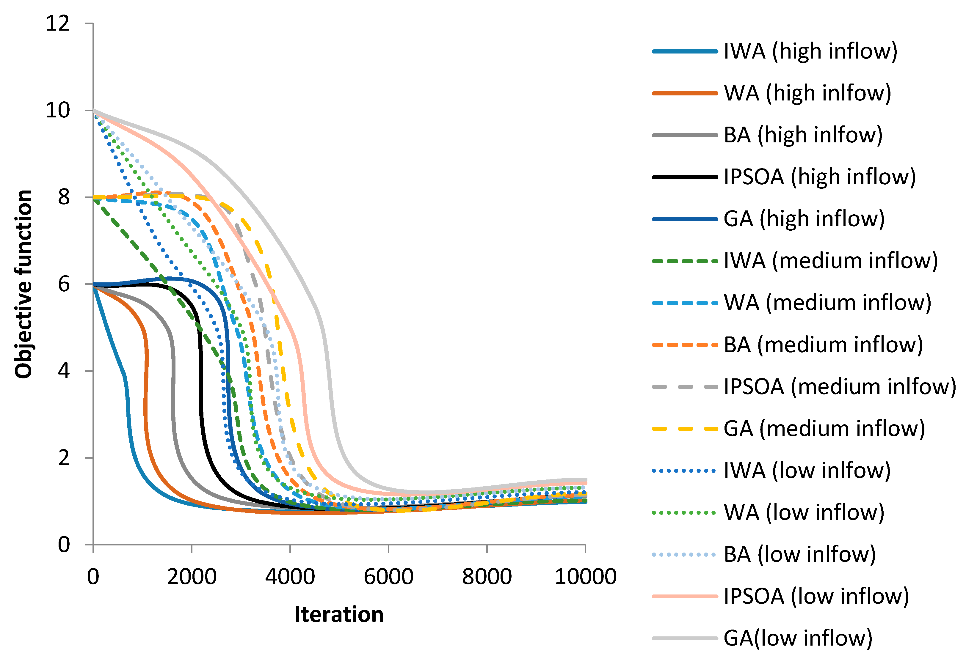
4.3. Convergence Curves for Different Algorithms

Figure 6, Figure 7 and Figure 8 shows the convergence curves for the different algorithms and inflows. At high inflow (Figure 6), after 1800 iterations, the IWA had converged while the WA, BA, IPSOA and GA converged after 2000, 2500, 3000 and 3000 iterations, respectively, indicating the IWA has the fastest convergence process among all the tested algorithms. The IWA converged after 3900 iterations for medium inflow while the WA, BA, IPSOA and GA converged after 4200, 4380, 4600 and 4800 iterations, respectively, (Figure 4). Figure 4 shows the fastest convergence was also for the IWA at low inflow.

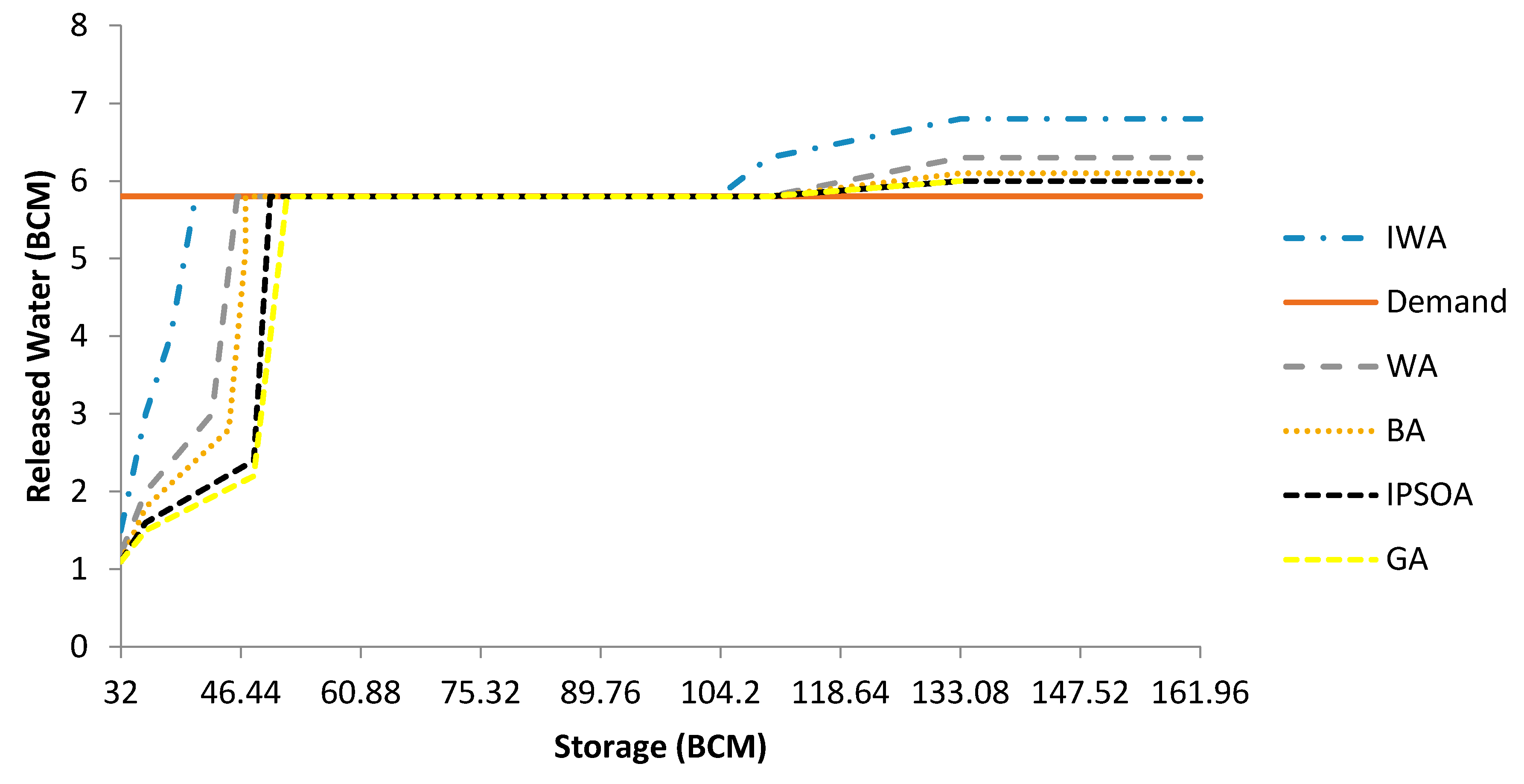
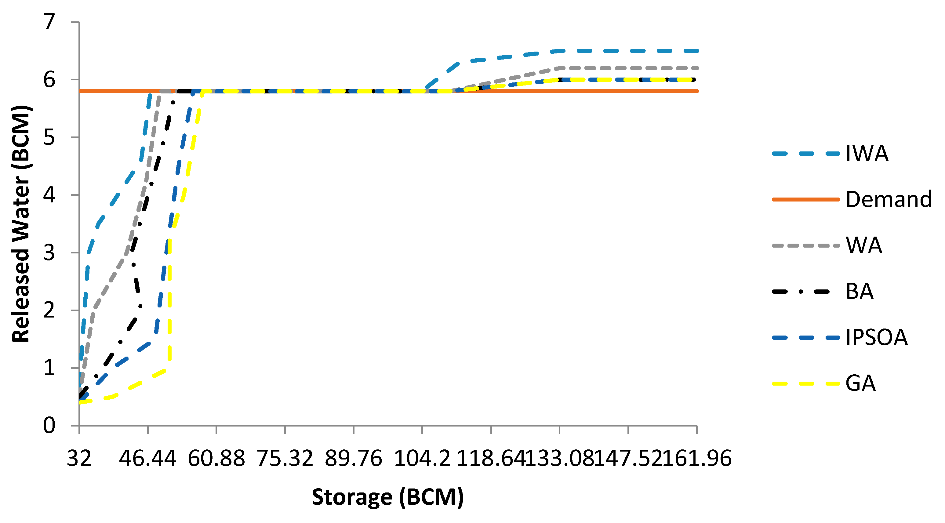
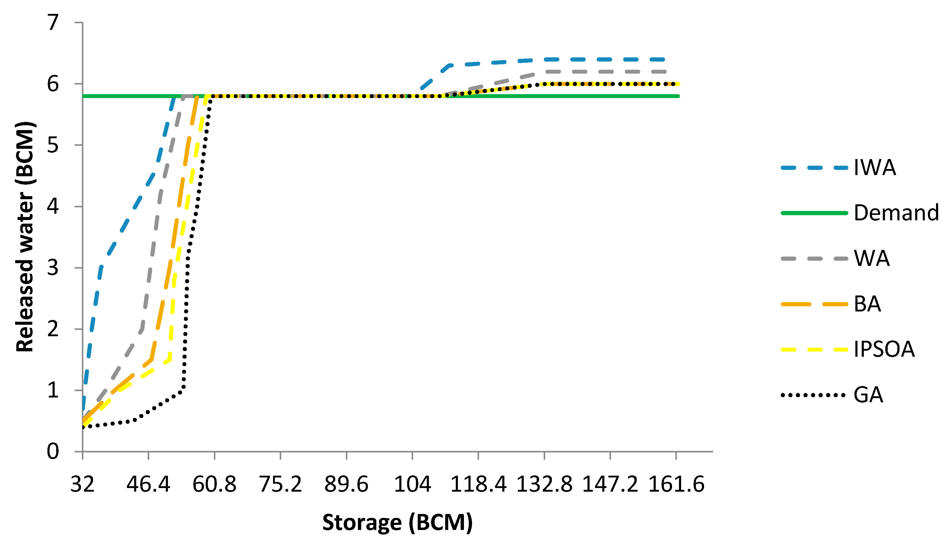
4.4. Analysis of Monthly Rule Curves for Reservoir Operation

Table 1 shows the average monthly inflows and demand during 1989 to 1999. July is the month with the greatest demand and therefore a critical month for analysis and avoiding of repetition of the same results. Figure 7 shows the average released water versus reservoir storage in July for 1989 to 1999 at high inflow. When the reservoir storage was 41 BCM, the released water could meet the demand (5.8 BCM) based on the IWA while the reservoir storage was 46, 47, 50 and 55 BCM for the WA, BA, IPSOA and GA, respectively, to meet the same demand. The IWA could therefore decrease reservoir storage at high inflow by about 10%, 14%, 18% and 25% compared to the WA, BA, IPSOA and GA, respectively. When the reservoir storage equaled 110 BCM at the high inflow using the IWA, the released water was greater than the demand (5.8 BCM) and could be used for the other needs such as power generation. At medium inflow (Figure 8), the IWA indicated that released water could meet demands with storage of 47 BCM, while the storage was 49, 52, 56 and 58 BCM for the WA, BA, IPSOA and GA, respectively. The IWA reduced storage for the demand supply by about 4.08%, 9.9%, 16% and 18% compared to the WA, BA, IPSOA and GA, respectively. In fact, the IWA can meet the demands earlier than WA, BA, IPSOA and GA. When storage calculated by the IWA at medium inflow was 112 BCM, the released water was greater than demand. For low inflow (Figure 9), the IWA indicated storage of 52 BCM was required to meet demands while the storage was 54, 55, 56 and 60 for the WA, BA, IPSOA and GA, respectively. The IWA reduced the storage for water supply at low inflow by about 3.7%, 5.4%, 7.6% and 14% compared to the WA, BA, IPSOA and GA, respectively. Figure 10 shows the released water for the different algorithms during 1989–1999 and the results indicated that the IWA met the demands more frequently than the GA, IPSOA, BA and WA. The reservoir storage for high inflow using the IWA was 41 BCM while for low and medium inflows it was 52 and 47 BMC, respectively. Thus, the storage should be increased for the low and medium inflows to satisfy the demands. A similar trend was noted for the other algorithms.

Table 9. Computed RMSE for low inflow.

$\mathit{R}\mathit{M}\mathit{S}\mathit{E}=\sqrt{\frac{{\left({\mathit{R}}_{\mathit{i}}-{\mathit{D}}_{\mathit{i}}\right)}^2}{\mathit{T}}},\mathit{T}:\mathit{N}\mathit{u}\mathit{m}\mathit{b}\mathit{e}\mathit{r}\left(\mathit{o}\mathit{f}\right)\mathit{p}\mathit{e}\mathit{r}\mathit{i}\mathit{o}\mathit{d}\mathit{s}(\mathbf{BCM})(\mathbf{Low}\mathbf{Inflow})$
Month	IWA	WA	BA	IPSOA	GA
January	1.32	1.43	2.12	2.18	2.30
February	1.21	1.31	2.11	2.15	2.55
March	1.12	1.14	1.65	1.78	1.79
April	1.14	1.16	1.78	1.82	1.75
May	0.98	1.02	1.22	1.45	1.57
June	0.91	0.93	0.98	1.14	1.21
July	1.56	1.57	1.59	1.61	1.52
August	1.11	1.21	1.14	1.16	1.18
September	1.12	1.14	1.15	1.17	1.21
October	0.76	0.78	0.82	0.85	0.87
November	0.012	0.015	0.017	0.019	0.020
December	1.14	1.21	1.31	1.32	1.30
Total	12.382	12.915	15.14	16.649	17.27
Medium Inflow
Month	IWA	WA	BA	IPSOA	GA
January	1.12	1.33	2.10	2.15	2.28
February	1.20	1.22	1.99	2.12	2.45
March	1.09	1.11	1.45	1.72	1.68
April	1.11	1.14	1.59	1.65	1.75
May	0.77	1.01	1.32	1.34	1.52
June	0.82	0.91	0.98	1.10	1.11
July	1.54	1.47	1.61	1.54	1.32
August	1.10	1.11	1.24	1.14	1.19
September	1.10	1.10	1.17	1.12	1.21
October	0.74	0.77	0.84	0.78	0.87
November	0.012	0.014	0.017	0.019	0.020
December	1.12	1.20	1.35	1.25	1.30
Total	11.83	12.51	15.657	15.925	16.7
Low Inflow
Month	IWA	WA	BA	IPSOA	GA
January	0.958	1.31	2.10	2.12	2.17
February	1.12	1.12	1.89	1.95	2.29
March	1.09	1.01	1.32	1.55	1.65
April	0.99	1.12	1.29	1.65	1.72
May	0.71	1.00	1.12	1.34	1.51
June	0.81	0.90	0.98	0.91	1.10
July	1.52	1.26	1.31	1.42	1.29
August	1.02	1.25	1.14	1.14	1.19
September	0.99	1.10	1.57	1.11	1.11
October	0.72	0.75	0.84	0.78	0.87
November	0.012	0.014	0.017	0.019	0.020
December	1.11	1.19	1.25	1.23	1.28
Total	11.05	12.024	14.827	15.390	16.18

shows the root mean square error (RMSE) between average released water with the demand value based on values in Table 1 for each month during the study period. Table 9 shows an RMSE for the low inflow using the IWA of 12.382 BCM, which was 4.1%, 18.21%, 18.69% and 28.3% lower compared to the WA, BA, IPSOA and GA, respectively. For the medium inflow (Table 9), the RMSE for the IWA was 11.38 BCM, which was 4.51%, 24.44%, 25.71% and 29.16% lower than the WA, BA, IPSOA and GA, respectively. Table 9 shows the same trend for high inflow. In other words, Figure 10 shows that the operation rule generated using IWA experienced more match between water released and demand.

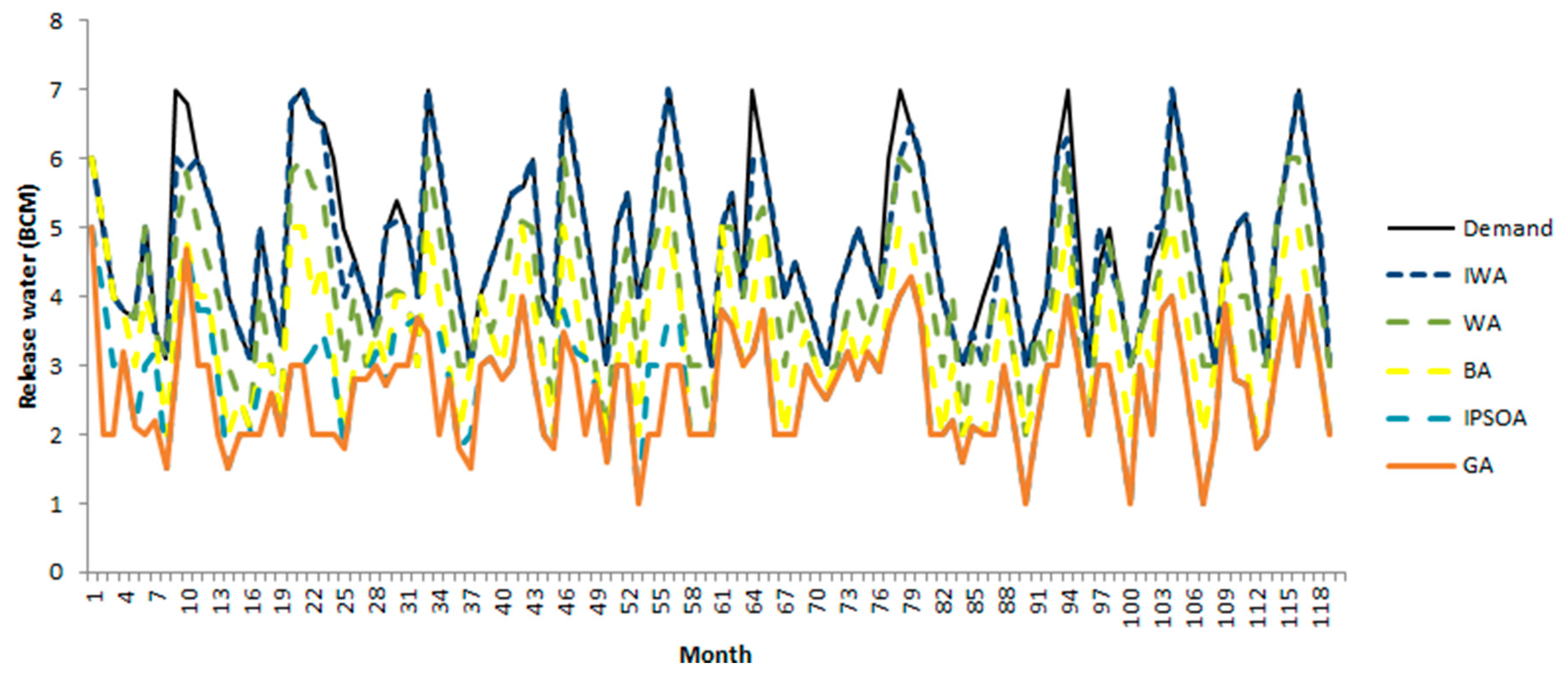
4.5. Analysis of Different Algorithms for Reservoir Operation during Total Operation Periods

Table 10. Computed different indexes for different algorithms

Algorithm	Reliability Index (%)	Vulnerability Index (%)	Resiliency Index
High Inflow
IWA	95	12	54
WA	91	14	52
BA	88	15	50
IPSO	78	17	49
GA	75	19	47
Medium Inflow
IWA	90	14	51
WA	89	16	50
BA	87	18	49
IPSO	74	19	48
GA	72	20	45
Low Inflow
IWA	89	16	50
WA	87	17	47
BA	85	20	44
IPSO	82	21	42
GA	70	22	40

shows the performance of the different algorithms for reservoir operation using the reliability, vulnerability and resiliency indices. The highest value for the reliability index for high inflow was 95% based on the IWA, which was 4%, 7%, 17% and 20% more than the WA, BA, IPSOA and GA, respectively. This indicated that the IWA could better supply the volume of demand compared to the other evolutionary algorithms. The reliability index for medium and low inflows based on the IWA were 90% and 89%, respectively, suggesting that at high inflow and based on the IWA, the reservoir could supply more of the demand.

For the IWA at high inflow, the vulnerability index was 12% while it was 14%, 15%, 17% and 19% for WA, BA, IPSOA and GA, respectively (Table 10). This meant that the intensity of failures for the reservoir operation based on the IWA was less than the WA, BA, IPSOA and GA and the system faced lower average deficits during the operational period (1989–1999). The system faced more deficits based on the IWA during the periods with low and medium inflows. Although the vulnerability index of the IWA was 2%, 4%, 5% and 6% lower for the medium inflow compared to the WA, BA, IPSOA and GA, respectively and 1%, 4%, 5% and 6% lower for low inflow, the vulnerability index based on IWA for medium and low inflow (14% and 16%) is 2% and 4% more than high inflow. Decreasing the inflow led to decreasing the volume of released water and thus, the system would face more deficits.

The highest value for the resiliency index at high inflow was for the IWA and it was 2%, 4%, 5% and 7% more than WA, BA, IPSOA and GA, respectively (Table 10). The resiliency index shows the model’s ability to recover from a critical period (failure). It is based on the ratio of the number of periods when reservoir water supply meets the demand to the number of periods when the demand is not supplied; thus, a high percent for this index is desirable. Although, the IWA acted better than the other evolutionary algorithms based on the resiliency index at all flows, the index declined from the high to lower flows. A similar trend was observed for the other algorithms. Figure 8 shows the released water for the different algorithms during 1989–1999 and the results indicated that the IWA met the demands more frequently than the GA, IPSOA, BA and WA.

5. Conclusions

The present study investigated the performance of an improved weed algorithm (IWA) and compared it to other evolutionary algorithms: the weed algorithm (WA), bat algorithm (BA), improved particle swarm optimization algorithm (IPSOA) and the genetic algorithm (GA). The operation of the reservoir of the Aswan High Dam, one of the most important dams in Egypt, was selected for this study. The IWA based on a local search operator attempted to improve the simple weed algorithm. Low, medium and high inflows to the reservoir were considered. The average solution by the IWA for low inflow was 1.121 and it was 0.30%, 0.90%, 2.9% and 5.4% less than the WA, BA, IPSO and GA, respectively. The computational time for the IWA at low inflow was 21s and was 3, 2, 6 and 7 s less than the WA, BA, IPSO and GA, respectively. Similar results were found for all three inflows. Based on extracted rule curves, the IWA could meet water demand earlier than the other algorithms. Using the IWA, reservoir storage was 41 BCM for the high inflow and the released water could meet the demand (5.8 BCM); the reservoir storage required was 46, 47, 50 and 55 BCM for the WA, BA, IPSOA and GA, respectively, to meet the demand at high inflow. The value of RMSE based on released water and demand was computed for each month and was less for the IWA than the other evolutionary algorithms. The vulnerability index for the IWA at high inflow was 12% while it was 14%, 15%, 17% and 19% for the WA, BA, IPSOA and GA, respectively. The reliability and resiliency indices were also better for the IWA at all three inflow rates compared to the other algorithms. The new weed algorithm has a high potential for solving different water resources management problems and it is suggested it can be used for multi-reservoir operation and multi-propose systems in future research. Although the method was used for Aswan High Dam but it can be used for other dams with the different applications because the method can supply the irrigation demands under different inflow conditions and thus, the method can be used for the dams with the aim of power generation on other demands. Some limitations for the methods are related to the accurate determination of random parameters that needs further research to accurate estimated utilizing advanced sensitivity analysis. In addition, even though the proposed model could be generalized to be applied for different case studies, it is recommended to the adaptation for the new case study constraints with the procedure of the IWA.

References

1. Srinivasan, K.; Kumar, K. Multi-objective simulation-optimization model for long-term reservoir operation using piecewise linear hedging rule. Water Resour. Manag. 2018, 32, 1901–1911. [Google Scholar] [CrossRef]
2. Ehteram, M.; Mousavi, S.F.; Karami, H.; Farzin, S.; Singh, V.P.; Chau, K.W.; El-Shafie, A. Reservoir operation based on evolutionary algorithms and multi-criteria decision-making under climate change and uncertainty. J. Hydroinform. 2018, 20, 332–355. [Google Scholar] [CrossRef]
3. Ahmadianfar, I.; Adib, A.; Salarijazi, M. Optimizing multireservoir operation: Hybrid of bat algorithm and differential evolution. J. Water Resour. Plan. Manag. 2015, 142, 05015010. [Google Scholar] [CrossRef]
4. Cheng, C.T.; Wang, W.C.; Xu, D.M.; Chau, K.W. Optimizing hydropower reservoir operation using hybrid genetic algorithm and chaos. Water Resour. Manag. 2008, 22, 895–909. [Google Scholar] [CrossRef] [Green Version]
5. Afshar, M.H. Large scale reservoir operation by constrained particle swarm optimization algorithms. J. Hydro Environ. Res. 2012, 6, 75–87. [Google Scholar] [CrossRef]
6. Chau, K.W. A split-step particle swarm optimization algorithm in river stage forecasting. J. Hydrol. 2007, 346, 131–135. [Google Scholar] [CrossRef] [Green Version]
7. Afshar, M.H. Extension of the constrained particle swarm optimization algorithm to optimal operation of multi-reservoirs system. Int. J. Electr. Power Energy Syst. 2013, 51, 71–81. [Google Scholar] [CrossRef]
8. Ehteram, M.; Karami, H.; Mousavi, S.F.; El-Shafie, A.; Amini, Z. Optimizing dam and reservoirs operation based model utilizing shark algorithm approach. Knowl. Based Syst. 2017, 122, 26–38. [Google Scholar] [CrossRef]
9. Fallah-Mehdipour, E.; Haddad, O.B.; Mariño, M.A. Real-time operation of reservoir system by genetic programming. Water Resour. Manag. 2012, 26, 4091–4103. [Google Scholar] [CrossRef]
10. Ostadrahimi, L.; Mariño, M.A.; Afshar, A. Multi-reservoir operation rules: Multi-swarm PSO-based optimization approach. Water Resour. Manag. 2012, 26, 407–427. [Google Scholar] [CrossRef]
11. Moeini, R.; Afshar, M.H. Extension of the constrained ant colony optimization algorithms for the optimal operation of multi-reservoir systems. J. Hydroinform. 2013, 15, 155–173. [Google Scholar] [CrossRef]
12. Zhang, Z.; Zhang, S.; Wang, Y.; Jiang, Y.; Wang, H. Use of parallel deterministic dynamic programming and hierarchical adaptive genetic algorithm for reservoir operation optimization. Comput. Ind. Eng. 2013, 65, 310–321. [Google Scholar] [CrossRef]
13. Haddad, O.B.; Moravej, M.; Loáiciga, H.A. Application of the water cycle algorithm to the optimal operation of reservoir systems. J. Irrig. Drain. Eng. 2014, 141, 04014064. [Google Scholar] [CrossRef]
14. Bozorg-Haddad, O.; Karimirad, I.; Seifollahi-Aghmiuni, S.; Loáiciga, H.A. Development and application of the bat algorithm for optimizing the operation of reservoir systems. J. Water Resour. Plan. Manag. 2014, 141, 04014097. [Google Scholar] [CrossRef]
15. Bolouri-Yazdeli, Y.; Haddad, O.B.; Fallah-Mehdipour, E.; Mariño, M.A. Evaluation of real-time operation rules in reservoir systems operation. Water Resour. Manag. 2014, 28, 715–729. [Google Scholar] [CrossRef]
16. Haddad, O.B.; Hosseini-Moghari, S.M.; Loáiciga, H.A. Biogeography-based optimization algorithm for optimal operation of reservoir systems. Water Resour. Plan. Manag. 2015, 142, 04015034. [Google Scholar] [CrossRef]
17. Asgari, H.R.; Bozorg Haddad, O.; Pazoki, M.; Loáiciga, H.A. Weed optimization algorithm for optimal reservoir operation. J. Irrig. Drain. Eng. 2015, 142, 04015055. [Google Scholar] [CrossRef]
18. Akbari-Alashti, H.; Haddad, O.B.; Mariño, M.A. Application of fixed length gene genetic programming (FLGGP) in hydropower reservoir operation. Water Resour. Manag. 2015, 29, 3357–3370. [Google Scholar] [CrossRef]
19. Bozorg-Haddad, O.; Janbaz, M.; Loáiciga, H.A. Application of the gravity search algorithm to multi-reservoir operation optimization. Adv. Water Resour. 2016, 98, 173–185. [Google Scholar] [CrossRef]
20. Ehteram, M.; Allawi, M.F.; Karami, H.; Mousavi, S.F.; Emami, M.; Ahmed, E.S.; Farzin, S. Optimization of chain-reservoirs’ operation with a new approach in artificial intelligence. Water Resour. Manag. 2017, 31, 2085–2104. [Google Scholar]
21. Ehteram, M.; Karami, H.; Mousavi, S.F.; Farzin, S.; Kisi, O. Optimization of energy management and conversion in the multi-reservoir systems based on evolutionary algorithms. J. Clean. Prod. 2017, 168, 1132–1142. [Google Scholar] [CrossRef]
22. Mousavi, S.F.; Vaziri, H.R.; Karami, H.; Hadiani, O. Optimizing reservoirs exploitation with a new crow search algorithm based on a multi-criteria decision-making model. JWSS 2018, 22, 279–290. [Google Scholar]
23. Karami, H.; Mousavi, S.F.; Farzin, S.; Ehteram, M.; Singh, V.P.; Kisi, O. Improved krill algorithm for reservoir operation. Water Resour. Manag. 2018, 32, 3353–3372. [Google Scholar] [CrossRef]
24. Ehteram, M.; Karami, H.; Farzin, S. Reservoir optimization for energy production using a new evolutionary algorithm based on multi-criteria decision-making models. Water Resour. Manag. 2018, 32, 2539–2560. [Google Scholar] [CrossRef]
25. Ehteram, M.; Karami, H.; Farzin, S. Reducing irrigation deficiencies based optimizing model for multi-reservoir systems utilizing spider monkey algorithm. Water Resour. Manag. 2018, 32, 2315–2334. [Google Scholar] [CrossRef]
26. Karami, H.; Ehteram, M.; Mousavi, S.F.; Farzin, S.; Kisi, O.; El-Shafie, A. Optimization of energy management and conversion in the water systems based on evolutionary algorithms. Neural Comput. Appl. 2018, 1–4. [Google Scholar] [CrossRef]
27. Roshanaei, M.; Lucas, C.; Mehrabian, A.R. Adaptive beamforming using a novel numerical optimisation algorithm. IET Microw. Antennas Propag. 2009, 3, 765–773. [Google Scholar] [CrossRef]
28. Rad, H.S.; Lucas, C. A recommender system based on invasive weed optimization algorithm. In Proceedings of the 2007 IEEE Congress on Evolutionary Computation, Singapore, 25–28 September 2007; IEEE: Piscataway, NJ, USA, 2007; pp. 4297–4304. [Google Scholar]
29. Chakraborty, P.; Roy, G.G.; Das, S.; Panigrahi, B.K. On population variance and explorative power of invasive weed optimization algorithm. In Proceedings of the 2009 World Congress on Nature & Biologically Inspired Computing (NaBIC), Coimbatore, India, 9–11 December 2009; IEEE: Piscataway, NJ, USA, 2009; pp. 227–232. [Google Scholar]
30. El-Shafie, A.; Jaafer, O.; Akrami, S.A. Adaptive neuro-fuzzy inference system based model for rainfall forecasting in Klang River, Malaysia. Int. J. Phys. Sci. 2011, 6, 2875–2888. [Google Scholar]
Figure 1. Production levels in the weed algorithm (WA).
Water 10 01267 g001
Figure 2. Improved weed algorithm (IWA) process.
Water 10 01267 g002
Figure 3. Bat algorithm (BA) process.
Water 10 01267 g003
Figure 4. Genetic algorithm (GA) process.
Water 10 01267 g004
Figure 5. Location and characteristics of Aswan High Dam.
Water 10 01267 g005
Figure 6. Convergence curve for low inflow, high inflow and medium inflow.
Water 10 01267 g006
Figure 7. Released water for high inflow.
Water 10 01267 g007
Figure 8. Released water for medium inflow.
Water 10 01267 g008
Figure 9. Released water for low inflow.
Water 10 01267 g009
Figure 10. Released water for the total of operation periods.
Water 10 01267 g010