Thermal and Hydrodynamic Changes under a Warmer Climate in a Variably Stratified Hypereutrophic Reservoir


1
Department of Geography, San Diego State University, San Diego, CA 92182, USA
2
Department of Forest Resources and Environmental Conservation & Virginia Water Resources Research Center, Virginia Tech, Blacksburg, VA 24061, USA
3
Department of Civil Engineering, Auburn University, Auburn, AL 36849, USA, [email protected]
*
Author to whom correspondence should be addressed.
Water 2018, 10(9), 1284; https://doi.org/10.3390/w10091284
Submission received: 24 July 2018
/
Revised: 9 September 2018
/
Accepted: 11 September 2018
/
Published: 19 September 2018
(This article belongs to the Section Urban Water Management)
Abstract
:We quantified effects of future climate warming on temperature and stability in a variably stratified, hypereutrophic reservoir with large fluctuations in water level by calibrating a 2-D model (CE-QUAL-W2, version 3.7.1, Portland State University, Portland, USA) of reservoir hydrodynamics using a time series (1992 to 2011) of inflow and air and water temperature. The model was then forced with increased air temperature projected by an ensemble of climate models that accounted for complex local topography and seasonality, with greater warming in summer. Warming increased annual evaporation rates by 2.6 to 7.9%. Water temperature increased by 0.44 (whole-reservoir; p < 0.05), 0.47 (epilimnion; p < 0.01), and 0.30 °C (hypolimnion; p < 0.05) per 1 °C increase in air temperature. Thickness of the epilimnion and hypolimnion diminished, with expansion of the metalimnion. Schmidt stability correlated with mean water depth over a wide range of depths (3.9 to 8.1 m; Adj. R2 = 0.91 to 0.93; p < 0.001). Increased air temperature increased mean annual stability by 6.1 to 23.6 J m−2 when depth was large and the reservoir stratified, but when depth was low (due to combined low inflow and, in preceding years, high withdrawals), inhibiting stratification, then water temperatures increased evenly (and more) throughout the vertical profile so change in mean annual stability was near zero (−0.1 to 1.1 J m−2). Combined effects of reservoir management (volume, timing, and elevation of water withdrawal) and climate warming (temperature of air and benthic sediment) can impact the hydrodynamic regime differently under variably stratified conditions with implications for release of phosphorus from sediment and vertical transport of phosphorus to the euphotic zone.
1. Introduction
Algal production, anoxia, and subsequent release of nutrients from benthic sediment are strongly controlled by timing, strength, and duration of thermal stratification. When a reservoir is stratified in summer, influx of dissolved oxygen (DO) from the atmosphere to the warmer epilimnion (with lower DO saturation) or from plant photosynthesis to the hypolimnion is limited and anoxia can occur when DO demand exceeds supply. Under anoxic conditions, ferric ions of iron reduce to the ferrous form, which leads to the dissolution of the phosphorus and iron bond and causes sediment to release soluble reactive phosphorus, iron, ammonia, and manganese to the hypolimnion [1]. Liberated phosphorus can be entrained to the euphotic zone through sustained vertical eddy diffusion, occasional entrainment, or annual mixis, resulting in increased algal growth. Decay and settling of algae into the hypolimnion and sediment feed microbial bacteria that have high DO demand, reinforcing a positive feedback.
Stratification, which is controlled in part by climate, has been altered in many systems by climate warming between 1970 and 2010 [2], and may be further impacted by future warming. Mean surface air temperature is projected to increase in the future [3], which may have opposing effects on stratification. Increased air temperature (and associated longwave radiation that enters a reservoir) heats a reservoir disproportionately at the surface, intensifying the vertical temperature gradient, increasing stability, extending the duration of stratification, and resulting in stratification at lower water levels [2,4,5,6,7,8], all of which increase the potential for anoxia and release of phosphorus from sediment [9]. Alternatively, increased evaporation rates and/or decreased inflow can lead to a long-term decrease in reservoir water depth, which can decrease stability and inhibit stratification if the reservoir is sufficiently shallow [6,10,11]. Most studies in the literature have investigated effects of climate warming on deeper reservoirs and lakes, which are monomictic or dimictic, but not variably stratified water bodies that are regularly or occasionally polymictic and have large intra-annual fluctuations in water level [2,4,5,6,7,12,13,14,15,16,17,18].
The objective of this study was to quantify the effects of a projected future warmer climate on thermal and hydrodynamic regimes in a reservoir that was intensively managed and became relatively shallow so that it ranged from being strongly to weakly stratified. Here, dam operators made decisions for volume, timing, and elevation of water withdrawal, which contributed to intra- and inter-annual variability in water depth and circulation. In turn, this complicated the determination of the parameters of the air temperature-stability relationship and the estimation of the impact of future warming on stability and duration of stratification. We calibrated a 2-D simulation model of reservoir hydrodynamics over a study period from 1992 to 2011, then forced the calibrated model with an ensemble of climate projections. We accounted for the effect of warming on other terms and feedbacks to the model in vertical (air temperature, precipitation, inflow, and benthic sediment) and lateral (inflow) directions.
The research questions were: What are the impacts of increased air temperature on water temperature, evaporation, and stability? How does warming impact the depth-stability relationship? How do impacts of warming differ when the reservoir is monomictic compared to polymictic? Are there seasonal differences in impacts of warming? We expected increased temperatures in all strata, with greater warming at the surface, which would increase stability for warmer climates. However, due to increased evaporation in a shallow reservoir with large surface area and concomitant lower water depth due to water withdrawal and management, we expected to see inhibition of stratification in some years of already low water level. We also expected greater magnitudes of change in water temperature and stability in summer compared to winter, given the extended period of high air temperature, high evaporation rates, and low precipitation rates typical during Mediterranean summers.
The study is of general interest as it tests a modeling framework for understanding how intensively managed and variably stratified reservoirs may respond to climate change. Intensively managed systems that have large seasonal changes in water level due to variations in both inflow and withdrawals may differ in their temperature-stability relationships compared with deep and natural lake systems. Management of intensively managed reservoirs is critical for municipal water supply, and understanding the impacts of climate change on their hydrodynamics and water quality is important for understanding potential climate-related risks to urban water resources.
2. Materials and Methods
2.1. Study Site
Hodges Reservoir (hereafter Hodges; Figure 1) supplies water for municipal use and is 50 km north of the city of San Diego, United States, and 20 km inland from the coast at an altitude of 70 m a.s.l. The reservoir basin is relatively shallow (8.5 m mean depth at capacity) compared to reservoirs in the region [11] and there is a relatively large interface between the hypolimnion and sediment, making it vulnerable to hypolimnetic anoxia and subsequent release of phosphorus from sediment [11,19]. At capacity, surface area is 6.0 km2 and maximum depth is 29.1 m. In most years, it is warm monomictic, but can be continuous warm polymictic when decreased inflow and/or increased drawdown inhibit stratification. Water level fluctuations were large over the study period, both intra-annually (mean amplitude = 3.5 m and maximum amplitude = 13.7 m) and inter-annually (maximum amplitude = 17.2 m), due to reservoir management, so stratification was controlled primarily by water depth and secondarily by air temperature [11].
Hodges is classified as hypereutrophic, as it had a high mean Anoxic Factor (AF; 157 day year−1), the number of days in a calendar year for which a sediment area equal to the surface area of a reservoir was overlaid with anoxic water (<1 mg DO L−1) [19], and the lowest Secchi disk transparency depth (1.0 m) relative to three other major water supply reservoirs in San Diego County [11]. Barrett, Morena, and Sutherland reservoirs had mean annual values of 161, 60, and 149 day year−1, respectively, for AF and 1.8, 1.7, and 1.2 m, respectively, for Secchi disk transparency depth over the study period. At Hodges, the mean hypolimnetic DO concentration was 0.1 mg L−1 and the reservoir became almost entirely anoxic due to algal production, decay, and related metabolic processes during mixis in autumn. The AF increased and transparency decreased while the frequency of winter events with near complete anoxia increased over the study period, which may be due in part to increased expansion of urban development in a watershed with significant agricultural land use [11].
Of all water entering Hodges between 1929 to 2010, local runoff accounted for 89%, imports for 5%, other inflows for 3%, and direct precipitation for 3%. There are four inflows to Hodges, all within close proximity of each other. The San Dieguito River contributes 92% of local runoff. It drains most of the Hodges watershed, which consists of mixed land use, including intensive and extensive agricultural, low-density residential, and open space. The balance (8%) of the local runoff to Hodges is conveyed by three streams (Felicita, Green Valley, and Kit Carson Creeks) draining smaller urban watersheds.
2.2. Study Design
We used CE-QUAL-W2 (hereafter W2; version 3.7.1, Portland State University, Portland, USA [20]), to simulate reservoir evaporation, water level, temperature, stability, and stratification from 1992 to 2011. These variables are impacted by simulations of the energy balance of the reservoir done by W2 using incoming solar radiation and longwave radiation estimated from air temperature, cloud cover, humidity, and wind data. We tested the sensitivity of the model to warming using the delta method, which adds a given temperature increase (∆T) to the observed historical time series of air temperature and uses the newly adjusted air temperature series as input to the model [21]. Our results include a reference run with no change, and runs for four warming scenarios.
Higher air temperatures increase conduction of heat from the atmosphere, and increase the temperature of precipitation, inflow, and sediment, all of which affect the energy balance of the reservoir. We accounted for higher temperatures of air, precipitation, inflow, and sediment in input data. We assumed relative humidity remains constant under a warmer climate; temperature of precipitation was set equal to daily mean air temperature; temperature of inflow was set equal to mean monthly air temperature over the study period [22,23]; and temperature of sediment was set equal to mean historical air temperature over the study period [20,24,25]. Although air temperature may not be a good estimate for temperature of precipitation due to a differential in elevation between where air temperature is measured and where precipitation forms, we assumed this assumption was justified due to the small proportion (3%) of precipitation relative to the total inflow that entered the reservoir. We set the temperature of sediment equal to the historical mean rather than to the mean of projected increased air temperature to allow for a temporal lag between air temperature and sediment temperature changes.
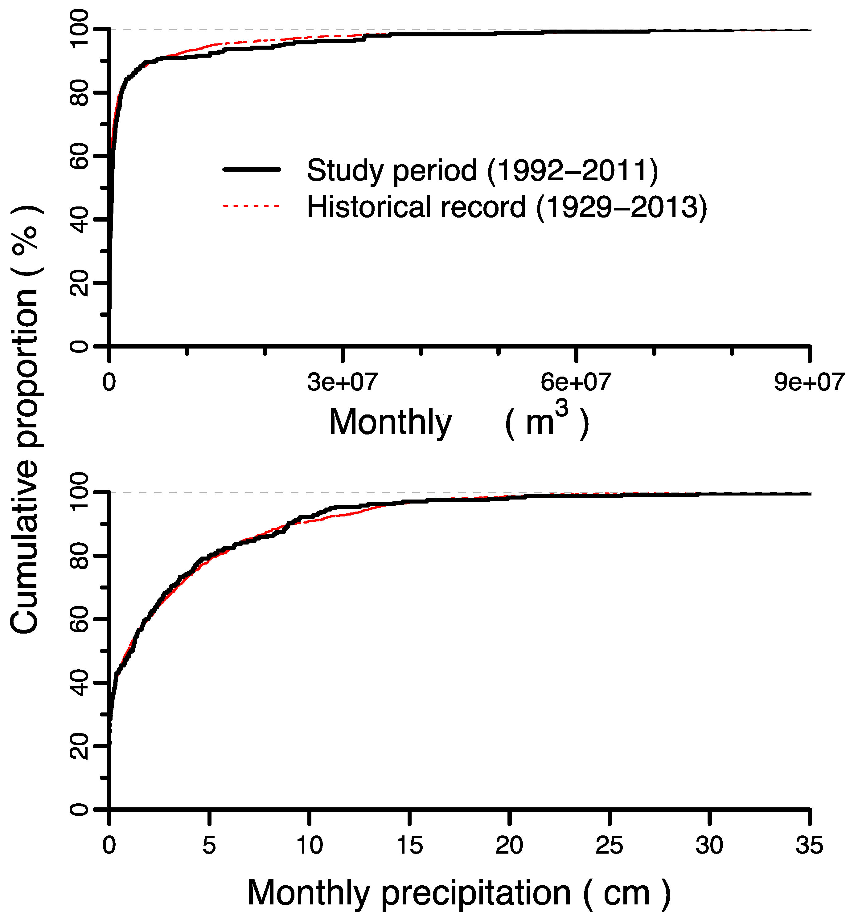
We did not consider explicitly how volume of precipitation or inflow may change due to climate warming because of a lack of consensus in the direction and magnitude of change in the literature. However, ranges of precipitation depth and inflow volume over the study period (1992 to 2011) were wide enough to be representative of the overall long-term historical record (1929 to 2013; Appendix A.1; Figure A1). Furthermore, almost all large precipitation events resulted in large runoff volumes, most of which (>90%) was spilled over the dam. Observed reservoir mean depth ranged from 3.6 to 8.5 m over the study period, including periods of overflow and an extended drought (2002 to 2004) when water levels were at record lows. Therefore, we simulated the response of the reservoir to both forecast climate (air temperature) scenarios and to a wide range of precipitation, runoff, and operation conditions.
2.3. Model Input and Calibration Data
The W2 model requires (1) daily time series of the volume and temperature of reservoir inflow and outflow (Appendix A.1); (2) bathymetric data to create depth-area-volume relationships (DAVR) for each model segment (Appendix A.2); and (3) daily time series of meteorological data (Appendix A.3). Water temperature profiles used for model calibration were taken at the deepest point near the dam at approximately 1 m depth intervals throughout the water column. Water temperature and Secchi disk transparency depth were measured monthly from January 1992 to November 2011 by City of San Diego.
2.4. Model Parameterization and Calibration
In low water years (2002 to 2004), when mean annual maximum depth, Z, <14.3 m and mean annual mean depth, , <4.5 m, observed stability was low and stratification did not develop. When water depths are low, sediment temperature becomes more tightly coupled with air temperature [24], most markedly during the spring and summer [26]. Our preliminary model runs showed that setting the sediment temperature equal to the mean of the historical daily mean air temperature artificially decreased the hypolimnetic temperature and artificially increased stability for warmer scenarios in low water years. Therefore, we divided the study period into smaller periods and modeled the summer (May to October) and the rest of the year (November to April) separately in low water years (Appendix A.4). For these low water years, we set the sediment temperature equal to the historical (no change run) or projected (warming scenario runs) mean of the daily maximum air temperature for the respective periods. Results for setting sediment temperature equal to the mean of the daily mean air temperature in low water years are reported to test for the impact of sediment temperature on the temperature profile of the water column.
Dam operations changed the elevation of water withdrawal from the middle of the water column in normal years to the bottom of the water column in low water years to ensure only less turbid hypolimnetic water was withdrawn for municipal water use [27]. The dam outlet structure is comprised of four downspouts (51 cm diameter cast iron pipes controlled by 51 cm gate valves) on the face of the dam for selective level draft control. Outlets are at the right side of the dam (looking downstream), not at the center line, and the overflow area is much shallower than other normal discharges. However, W2 is a two-dimensional model and does not fully reflect the three-dimensional flow dynamics. Preliminary model runs showed poor fits in the temperature profiles, particularly when the reservoir was observed to be isothermal in low water years. These poor fits led to simulated stratification when none was observed. Therefore, we raised the upper withdrawal elevation by 1.7 m to 88.3 m a.s.l and lowered the lower withdrawal elevation by 4.8 m to 72.6 m a.s.l, which improved model fit substantially, particularly in low water years. We determined that outlet elevation was the most impactful and sensitive parameter that could explain why the shapes of the temperature profile were modeled to be either isothermal (which matched observations) or stratified (which was erroneous) in low water years. The shapes of the profile could not be corrected by adjusting any other parameters (e.g., coefficients of sediment heat transfer, wind sheltering, or shading). There may be some discrepancies in the model bathymetry and other bathymetric data used to build the model due to sedimentation (Appendix A.2).
The model was further calibrated by adjusting radiation and wind coefficients until the model matched well with observed water levels and profiles of water temperature. Short-wave solar radiation was reduced by a static shade coefficient, which was calibrated to 0.94 [20], meaning that 94% of the incoming short-wave solar radiation was allowed to reach each surface segment. A shade coefficient was ideal for modeling a long, narrow reservoir, such as the study reservoir, which is in a canyon and surrounded by rolling hills. In low water years, shading increased and the value of the shading coefficient was calibrated to 80%. Radiation penetrates the surface of the water, heating the water column, and decays exponentially with depth, according to Beer’s Law:
where Hs(Z) is short-wave radiation (W m−2) at depth Z (m), βS is the fraction absorbed at the water surface, Hs is short-wave radiation reaching the surface (W m−2), e is the base of the natural logarithm, and η is the radiation extinction coefficient in the water column (m−1). The extinction coefficient, η, was estimated for each observation of Secchi disk transparency depth, ZSD:
where K is a constant, 1.7 [28,29]. Secchi disk transparency depth was chronically low (mean = 1.0 ± 0.05 m) over the study period so the mean extinction coefficient value was 2.3 (± 0.1) m−1, which was typical for a eutrophic system, in which values can range from 0.5 to 4.0 m−1 [30]. Monthly values for the extinction coefficient were linearly interpolated to daily values for the study period. The coefficient calculated in this approach empirically accounted for total radiation extinction due to the combination of, for example, pure water, algae, suspended solids, zooplankton, and macrophytes. We did not model any biological processes using W2 to isolate the abiotic effects of warming on the study reservoir and to reduce the number of parameters for which we did not have data.
Hs(Z) = (1 − βS) Hs × e−ηZ
η = K/ZSD
The evaporative wind speed function, f(W), in W m−2 mm Hg−1, is given as:
where a, b, and c are default empirical coefficients (9.2, 0.46, and 2, respectively) [31] and W is wind speed measured at 2 m above the ground (m s−1) multiplied by the wind sheltering coefficient. Water levels and temperature profiles were insensitive to the wind sheltering coefficient and so the wind coefficient was set to 1.00, meaning that wind speed was not changed from observed values.
f(W) = a + bWc
Model fit was determined visually and statistically. After the general shape (e.g., straight versus curved) in a temperature profile was inspected and determined to be correctly simulated, then the more precise differences between the modeled and observed temperature profiles were quantified using the absolute mean error (AME) and root mean square error (RMSE), given as:
where Xi is the ith temperature (°C) and n is the number of observations in a profile. The AME is the average absolute deviation between modeled and observed temperature in degrees (°C) and we considered an AME of 1 °C or below to be a good fit [20]. The AME and RMSE have been used to assess the accuracy of W2 models in other studies [20].
2.5. Climate Warming Scenarios
The calibrated model was run with no change (NC) for reference, then with ∆T taken from four projections of mean air temperature for 2035 to 2064. Projections were made by the Parallel Climate Model (PCM) from the National Center for Atmospheric Research and Department of Energy, and the Geophysical Fluid Dynamics Laboratory CM2.1 model (GFDL) from the National Oceanic and Atmospheric Administration. The models were selected because they produced a more realistic representation of local climate, accounting for diverse topography and Mediterranean seasonality [32]. Projections were made for low (B1) and medium-high (A2) CO2 emissions scenarios [33], resulting in four climate warming scenarios (PCM.B1, PCM.A2, GFDL.B1, GFDL.A2; Table 1). These warming scenarios are referred to hereafter in increasing order of warming as Scenario 1 (PCM.B1), Scenario 2 (PCM.A2), Scenario 3 (GFDL.B1), and Scenario 4 (GFDL.A2). The B1 emission scenarios assumed that CO2 emissions will reach a maximum of ~12 GtC year−1 in 2050 before dropping below ca. 2000 levels to 5.2 GtC year−1 by 2100. The A2 emission scenarios assumed that CO2 emissions will increase throughout the century to ~29 GtC year−1 by 2100. Cumulative CO2 emitted from 1990 to 2100 varied from 989 (B1) to 1773 (A2) GtC.
2.6. Data Analysis
2.6.1. Reservoir Temperature and Stability
Volume-weighted water temperature was calculated for the whole reservoir (TR), epilimnion (TE), and hypolimnion (TH) for each observed and modeled water temperature profile. The thermocline was defined as the horizontal plane of the maximum temperature gradient, with a minimum of 1 °C m−1, in the vertical water column [34]. The lower boundary of the epilimnion was defined as the deepest depth above the thermocline where the temperature gradient between adjacent strata was less than 0.5 °C m−1 and the upper boundary of the hypolimnion was defined as the shallowest depth below the thermocline where the temperature gradient between adjacent strata was less than 0.5 °C m−1. The metalimnion was defined as the water body in between the epilimnion and hypolimnion.
Stability was quantified using the Schmidt Stability Index, S (J m−2), which is the minimum amount of work that must be done by wind to return a reservoir to an isothermal state, calculated from differences in water density in the water column [35]:
where g is acceleration due to gravity (m s−2), A0 is surface area of the reservoir (m2), AZ is reservoir area (m2) at depth Z (m), ρZ is water density (kg m−3) at depth Z, ρ* is mean water density (kg m−3) of the reservoir, and Z* is the depth (m) where the mean water density occurs. The summation is taken over all depths at approximately 1 m intervals, dZ, from the surface to the maximum depth, Zm. Water density, ρ (kg m−3), was calculated as a function of temperature, T (°C), using the Thiessen-Scheel-Diesselhorst Equation [36].
Hodges was defined as thermally stratified when there was development of a thermocline and when S exceeded 100 J m−2. Linear interpolation of S between observation dates was used to determine dates of onset of stratification and turnover. Results were aggregated to means for the calendar year (January to December) and non-stratified winter period (November to March).
2.6.2. Multiple Regression Models of Controls on Temperature and Stability
Multiple regression was used to identify the controls on changes in water temperature and stability that resulted from climate warming. Minimal adequate regression models of stability and water temperature were determined through forward and backward stepwise variable selection. Backward selection was an iterative process of deleting the least significant term in a maximal model until remaining terms were significant (α = 0.05). An appropriate model was selected based on explanatory power (R2), plausibility given physical processes, and parsimony. The relative contribution to R2 from each term, alone and in combination with others, in a model was based on sequentially determined R2 values, which depended on the order in which terms were entered into a regression. To control for the sequence of addition, the unique contribution to R2 for an explanatory variable was given by the Lindeman, Merenda, and Gold statistic (LMG) [37,38]. The statistic can be interpreted as the average squared semi-partial correlation coefficient for a regressor, which is determined as the average of all possible permutational orderings of that regressor within the set of all regressors.
3. Results and Discussion
3.1. Model Calibration
Observed and modeled water depths (Z) under historical climate and hydrologic conditions were generally in good agreement (Figure 2). W2 correctly simulated water depth during most reservoir filling events and extended periods of drawdown and evaporation. However, an underestimation for the fill event in 1998 may have led to an underestimation in depth between 1998 and 2003.
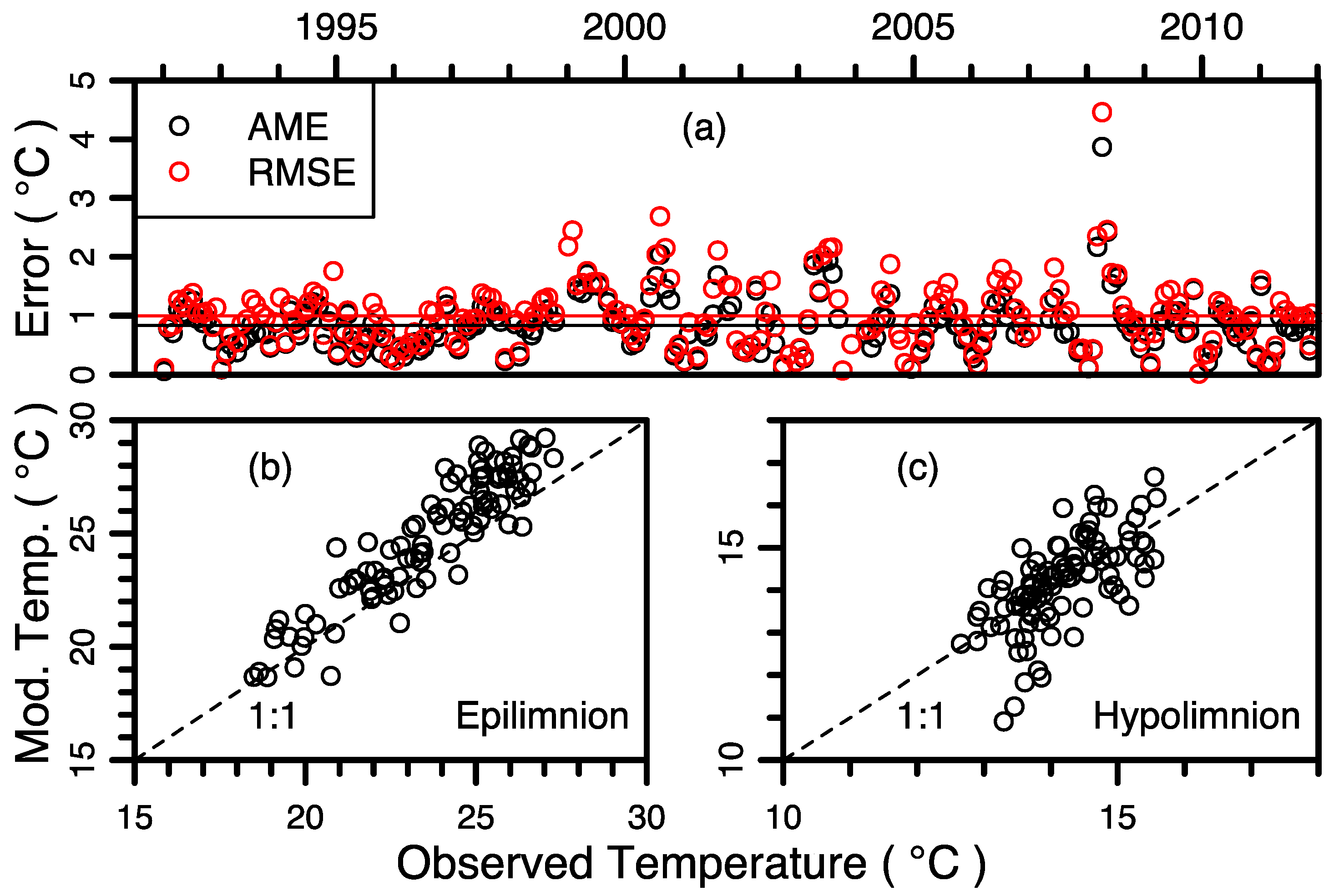
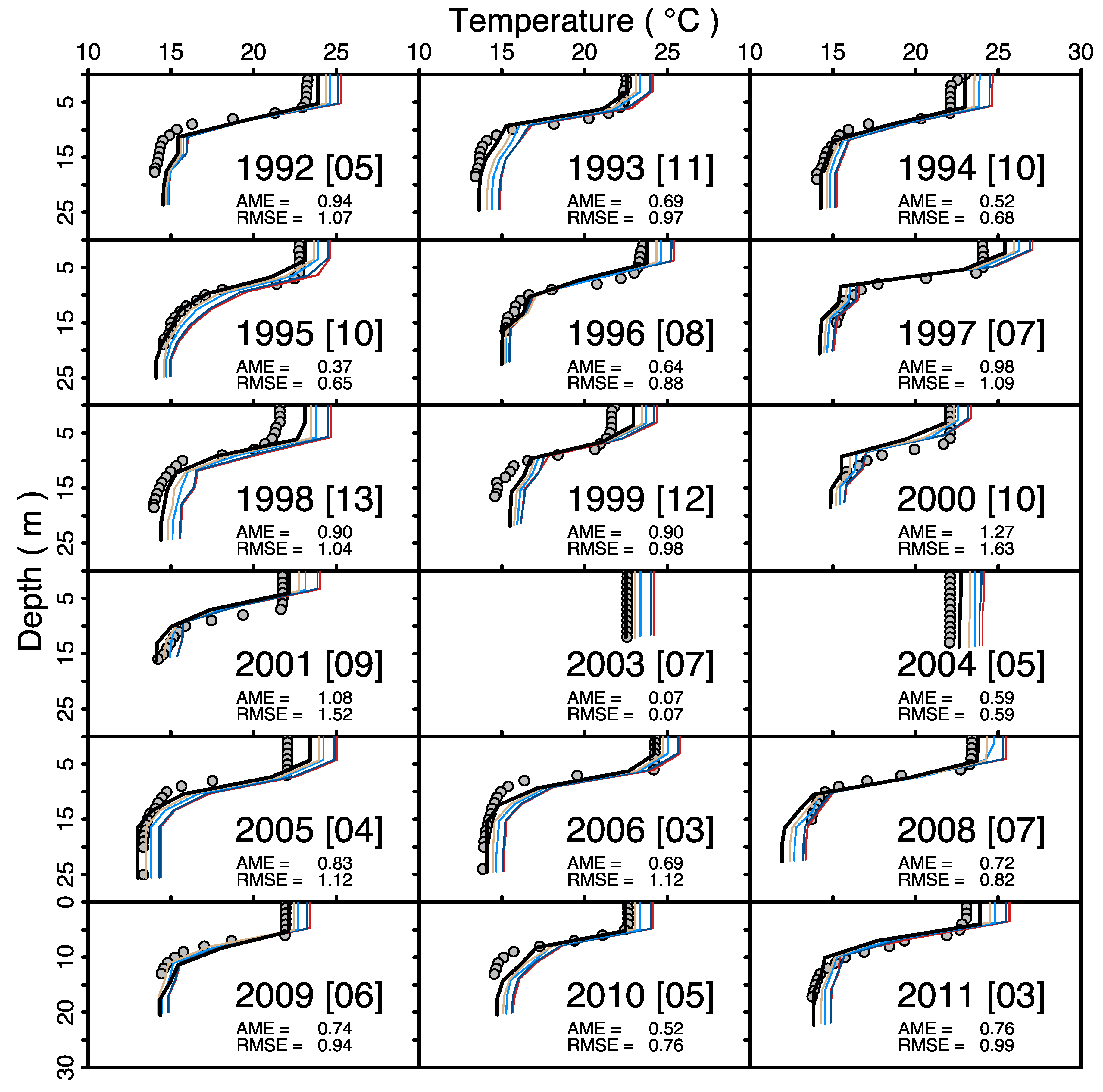
Observed and modeled temperature profiles under historical conditions with no change were in good agreement (Figure 3, Figure 4 and Figure 5). The profile’s AME was typically below 1 °C in most months (Figure 3a). The AME was 0.84 ± 0.03 °C when averaged over the entire study period, and similar (0.78 ± 0.10 °C) for low water years (Figure 3a), confirming that W2 adequately modeled temperature for highly variable water levels. Observed and modeled epilimnetic and hypolimnetic temperatures were significantly correlated (p < 0.001), with Adj. R2’s of 0.83 and 0.42, respectively (Figure 3b,c). Monthly temperature profiles for a typical year (1995) with normal water levels are presented in Figure 4 to show the model fit to observed profiles and forecast warming of water temperature due to four projected scenarios (Table 1). When the sediment temperature was set equal to the mean of daily mean air temperature in the low water years, the shapes of the temperature profiles were erroneous, particularly in the (observed) isothermal hypolimnion in September and October, and mean AME was higher (0.95 ± 0.14 °C), suggesting that the mean of daily maximum (instead of mean) air temperature was a better assumption for sediment temperature in low water years. Temperature profiles in the month of October (1992 to 2011) are presented in Figure 5 to show the consistency of the model in simulating stratification over the study period and also to show the robustness of the model in simulating the contrasting temperature profiles in low water years, when the reservoir did not stratify and the sediment temperature was set to the mean of daily maximum air temperature.
3.2. Higher Rates of Evaporation under Warming Scenarios
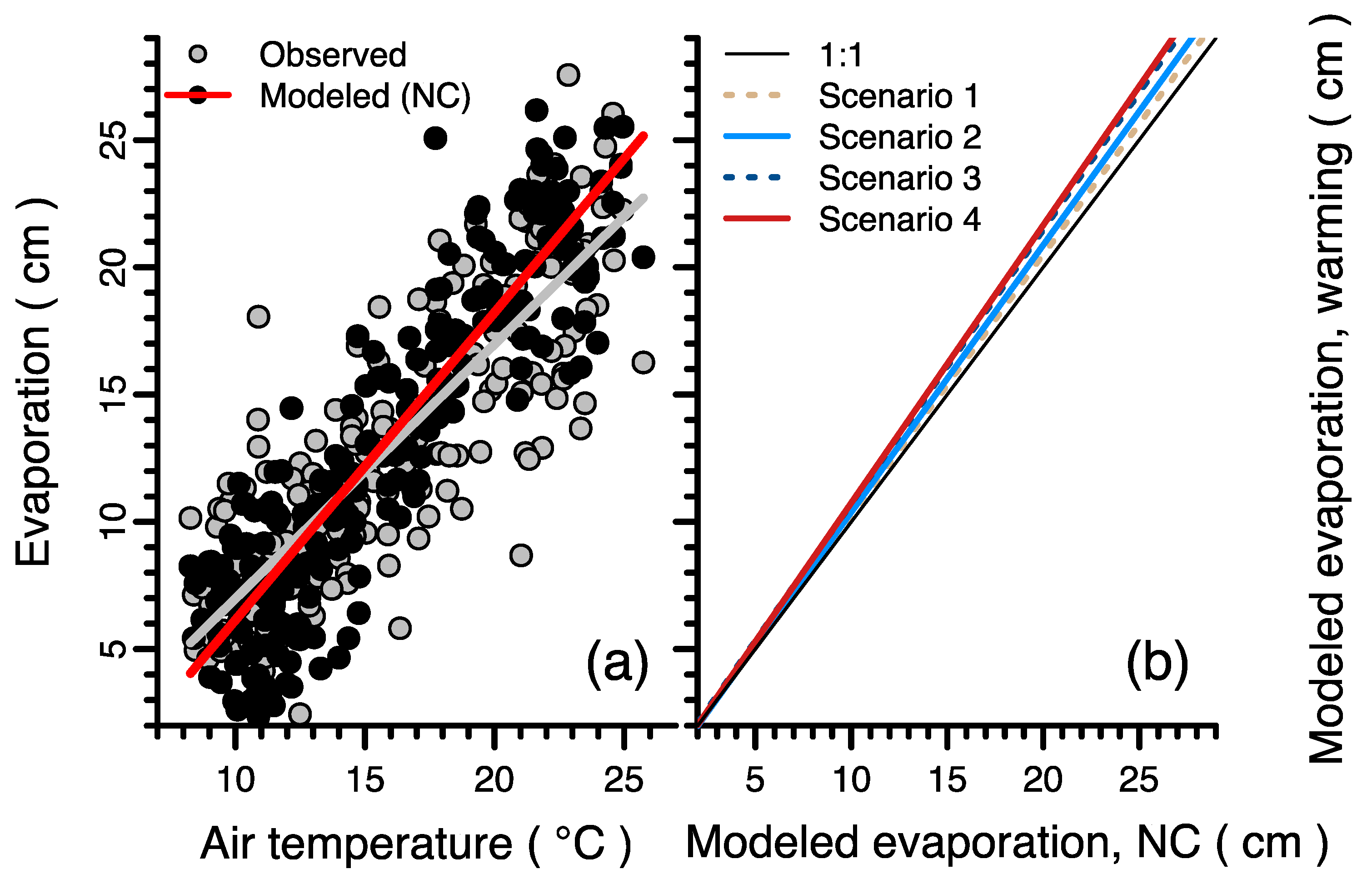
Observed and modeled evaporation (E) under historical conditions were significantly correlated (Adj. R2 = 0.71; p < 0.001; Figure 6a) and mean annual averages for the study period were similar (EOBS = 154.0 cm year−1; EMOD = 159.0 cm year−1). Evaporation increased by 2.6 to 7.9% for all warming scenarios relative to the reference run (EScenario1 = 163.1; EScenario2 = 165.5; EScenario3 = 170.6; EScenario4 = 171.6; all units cm year−1), which was comparable to the average increase (3.6%) projected across 47 reservoirs in California under similar climate forcing [39]. Though the impact of these increases in evaporation is small for deeper water bodies, it can be substantial in shallower reservoirs, including the study reservoir, during years with low water levels ( < 4.5 m).
Increased evaporation due to warming reduced modeled by 0.04 to 0.09 m (Table 2), averaged over the study period, after removing data from low water years. Modeled reductions in depth under a warmer climate were ~3 times larger during low water years due to higher evaporation rates, continued withdrawals for urban use, and the rapid rate of change in depth for a given change in volume at low water depths. Higher rates of E during low water years were plausible because water temperature, net radiation, and the vapor deficit were all higher in those years. The temperature of the whole reservoir was observed and modeled to be ~1 °C higher in low water years than in normal years (Table 2). The bathymetry of the reservoir is such that depth changed slowly for a given volume change at high water depths but rapidly at low water depths, so withdrawals for urban use had a larger impact on depth when Z was low (Figure 2).
3.3. A Warmer Thermal Regime
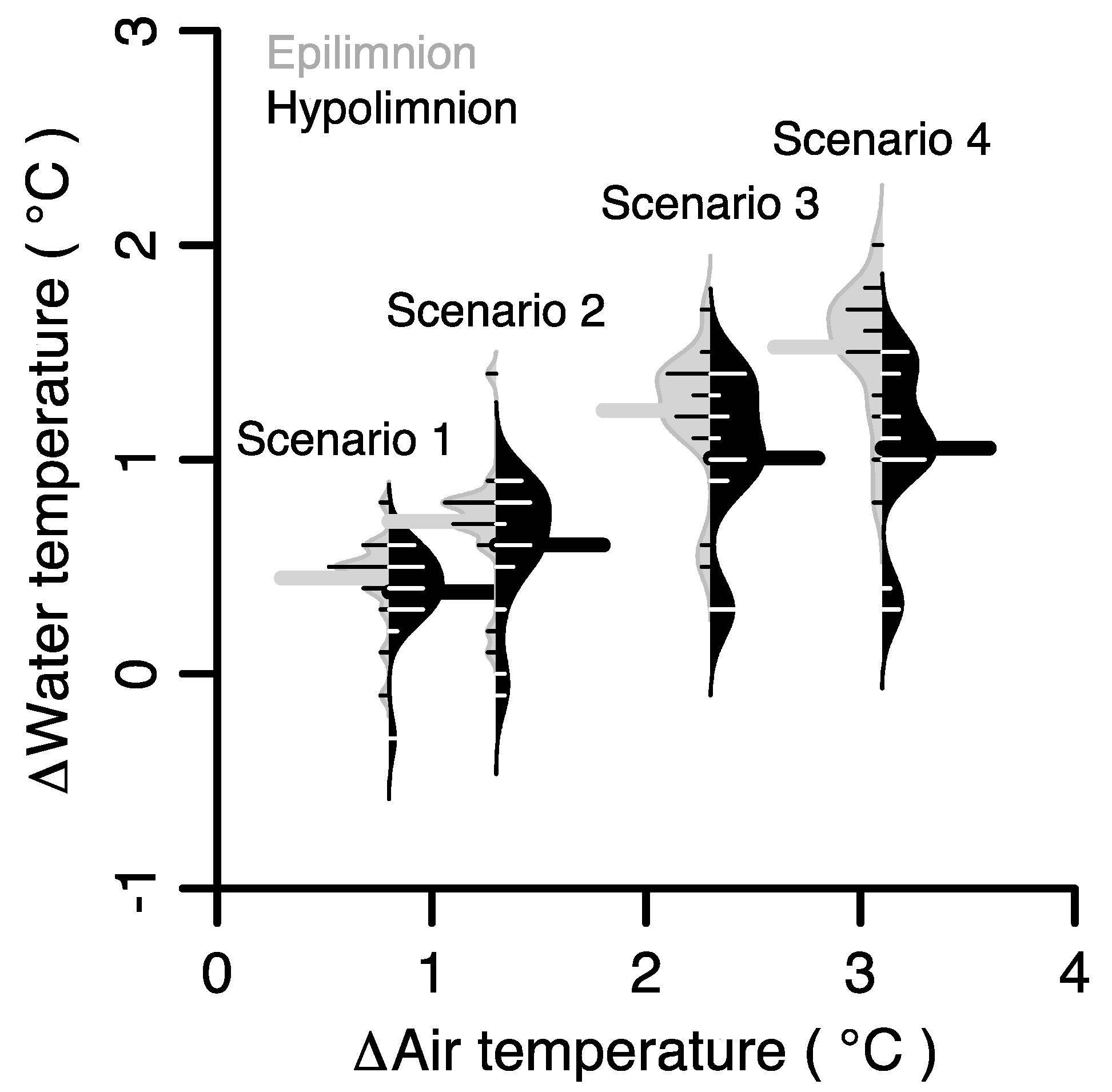
There was a strong coupling of air and water temperatures throughout the profile. Annual weighted-average warming of air temperature (TA) by 0.8 to 2.4 °C increased water temperature by 0.5 to 1.5 °C, on average, in the whole reservoir (Table 2) and epilimnetic and hypolimnetic temperatures increased significantly with increasing air temperature across scenarios (Figure 7). Increases in water temperatures were larger for warmer scenarios. Regressions showed that a 1 °C increase in summer air temperature corresponded with an increase of 0.44 °C in the whole reservoir (TR = 0.18 + 0.44 × TA; Adj. R2 = 0.94; p < 0.05; Figure 7), 0.47 °C in the epilimnion (TE = 0.09 + 0.47 × TA; Adj. R2 = 0.99; p < 0.01), and 0.30 °C in the hypolimnion (TH = 0.19 + 0.30 × TA; Adj. R2 = 0.89; p < 0.05). Both whole-reservoir temperature averaged over the year (TR) and over winter (TR-W) increased more in warmer scenarios (Table 2). Contrary to initial expectations, increases in TR-W were similar to increases in TR in all warming scenarios.
Changes in TE explained the majority of variance in the changes in TH in a warmer climate (LMG = 0.66) and changes in hypolimnetic thickness (LH) explained little variance (LMG = 0.03; Table 3), which showed the importance of the epilimnion in mediating warming of the hypolimnion. In a relatively shallow reservoir, heating of the hypolimnion is not directly related to meteorological forcing by itself [5] but is rather a complex interaction between energy exchanges between the epilimnion and hypolimnion, which is mediated by mixing and stratification. Furthermore, heating of the hypolimnion is due primarily to warming from the atmosphere and downward transfer of heat through convection from the epilimnion [40], rather than to secondary sources of heating, including precipitation, inflow, and benthic sediment. The total input of heat to the reservoir increased under warming, but heat at the surface increased resistance to mixing, reducing the downward movement of heat across the thermocline [8].
3.4. Stability and Stratification
Mean annual stability (S) increased by 6.1 to 23.6 (J m−2) in normal years, by less in the winter (SW; 2.6 to 8.0 J m−2), and by near zero in low water years (SNS; −0.1 to 1.1 J m−2), all with generally larger increases for warmer scenarios (Table 2). In normal years, the duration of stratification increased for all warming scenarios by 6 to 14 days, with the onset of stratification moving earlier in the year by 4 to 9 days on average over the study period (Table 2). W2 correctly simulated the low stability and observed inhibition of stratification in low water years in the reference run. Stratification did not occur during these years in any of the warming scenarios, either.
Increases in S were dampened both in the winter and in low water years because the water column was isothermal. Stability increased less in low water years than in the winter of normal years because of a warmer and shallower water column. In low water years, water temperature was initially high due to preferential removal of colder hypolimnetic water through a lower elevation outlet, rather than due to heating from the air. Also, there was likely a larger influence from warmer benthic sediment on warming of the hypolimnion when the water level was low. This suggested that when the water level was low, air temperature, which we assumed impacted sediment temperature, had opposing impacts on S depending on the relative changes at the top and bottom of the temperature profile.
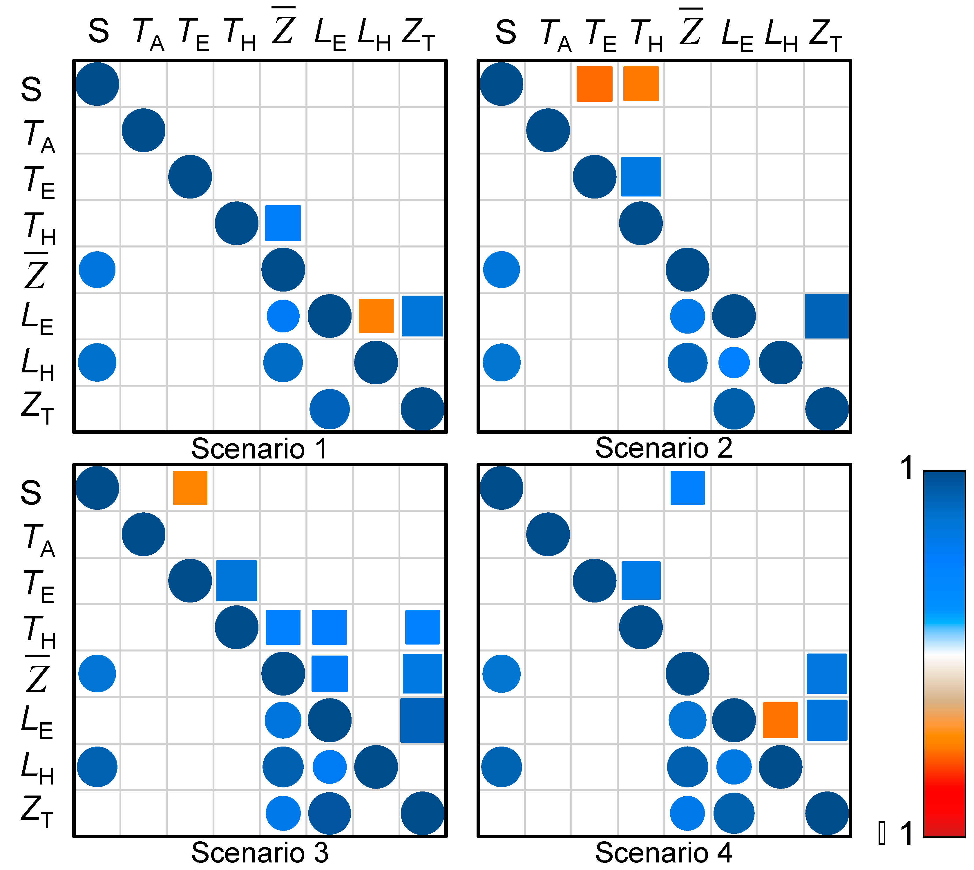
To understand the impact of climate warming on stability in normal years, we did separate correlation analyses between relevant reservoir variables. In Figure 8, circles are correlations between metrics under the changed climate in a management-dominated system where water level fluctuations were the primary control on hydrodynamics. In the same figure, squares are correlations between changes in metrics after climate warming relative to the reference run (with no change). The squares in Figure 8 were calculated as the correlations of the differences in the values of a given variable between the given warming scenario and the reference run. This analysis held water level fluctuation and management constant and showed only the impact of increased air temperature (and related variables) on reservoir metrics.
In the management-dominated system, S consistently correlated with and LH (Figure 8 circles), but in the climate-modified system, S did not consistently correlate with any single variable (Figure 8 squares). Multiple regression results showed that changes in TA, , and TH together explained the change in S (Adj. R2 = 0.86; Table 3). This suggested that increased TA (LMG = 0.67) and E, which also directly impacted (LMG = 0.09), were important and significant predictors of changes in S. Air temperature increased the slope of the depth-stability relationship, and mean annual stability was higher for all depths in warmer scenarios, with increased stability for warmer scenarios (Figure 9).
Climate warming changed the distribution of heat in the water column. Changes in depth and heat distribution in the profile (epilimnetic thickness LE, LH, and thermocline depth ZT) were highly correlated with each other (Figure 8 squares). The metalimnion expanded as LE, LH, and ZT decreased on average in all scenarios over the study period, with larger decreases in LE, LH, and ZT in warmer scenarios (Table 2). Thermocline depth has increased in many lakes in response to climate warming [2]. In contrast, in the study reservoir ZT decreased likely due to factors including lower water depth due to increased E, and high turbidity, which limited penetration of light and heat, as observed in other reservoirs [8,41]. Future research could model the impact of allochthonous nutrient supply and climate warming on algal production and the resulting direction of change in ZT.
3.5. Implications of Changes to the Hydrodynamic Regime
Higher air temperatures increased water temperature throughout the profile and throughout the year (Figure 4). The change in temperature has implications for other water quality parameters. Increased water temperature decreases DO saturation. At water temperatures around 14 °C (mean observed TH; Table 2), the DO saturation decreases by about 0.20 mg L−1 per one degree of increase in water temperature. Hence, the DO saturation would decrease by approximately 0.06 mg L−1 for the expected 0.30 °C increase in hypolimnetic water temperature, per one degree in the air temperature (Figure 7). Warmer water has been shown to correlate with increased sediment microbial metabolism [42], hypolimnetic anoxia [5], and release of phosphorus from sediment [43].
Warmer climate had variable impacts on the hydrodynamic regime of the reservoir, depending on its depth. Warmer climate increased stability and extended the duration of stratification in normal years. The combination of increased water temperatures and stability can favor nuisance cyanobacteria, increasing their ambient biomass levels and the frequency and persistence of blooms [41]. However, hydrodynamic conditions were different in low water years, due primarily to management (i.e., volume, timing, and elevation of water withdrawal) removing colder hypolimnetic water. Under low depth conditions, the reservoir became isothermal, essentially behaving as a well-mixed epilimnetic layer, and the magnitude of increase in stability from climate warming was near zero. The reservoir became sufficiently shallow that solar radiation penetrated deeper through the water body than when water level was higher, which led to higher water temperatures and evaporation rates compared with normal years. Water temperature and evaporation rates may be more impacted by climate warming due to additional processes of sediment warming in reservoirs that are actively managed and have shallower depths.
Sediment can heat or cool the hypolimnion seasonally [40] so the timing of equilibration of sediment temperature to air temperature has important effects on stability and mixing of nutrients. Equilibration appeared to be rapid in low water years, but, in early model runs when assuming instant equilibration in normal years (sediment temperature = air temperature), average warming of the hypolimnion was higher than of the epilimnion (causing smaller increases of stability), which suggested that sediment was a net heat source in the model. This seemed physically implausible because sediment does not produce heat and sediment heat exchange with water is small compared to surface heat exchange [20]. Therefore, we reported results from when sediment temperature was set equal to the historical air temperature record, recognizing that we likely underestimated sediment temperature in warming scenarios, which could result in an underestimate of warming of the hypolimnion and overestimate of stability. These findings demonstrate the importance of sediment-water energy exchange, particularly in shallower reservoirs, and future work in such systems should simulate dynamic sediment temperature and its interactions with the water column [24].
In low water years with low stability, it was possible that release of phosphorus from sediment may still have occurred, despite the lack of long-term stratification, which can result in enhanced mixing and increased delivery of nutrients to the euphotic zone. It is known that in a polymictic reservoir, short periods of stratification, on the order of hours or days, may occur [44] and cause sediment release of phosphorus if there are conditions of low DO and high rates of oxygen reduction at the sediment-water interface [45]. The study reservoir showed perennially low hypolimnetic DO concentrations during the study period [11], and previous studies report low DO concentrations after mixis in December [46] and heterograde DO profiles when the reservoir was isothermal in January [47], indicating that the hypolimnion was rich in nutrients and could support production through winter. When depth and stability are low, algal production can then be supported by vertical transport of hypolimnetic and sedimentary nutrient reserves released from the sediment [48] and exposed littoral zone [49,50]. Sediment can be in constant contact with the euphotic layer and phosphorus concentrations can remain high because of the lack of water to dilute those concentrations in that layer.
This study provides an example of a managed system in which air and water temperatures were tightly coupled, so that abiotic climate warming significantly exacerbated changes in water level and, in turn, stability. Inhibition of stratification due to forecast warmer climate is projected to turn lakes from a dimictic to monomictic regime in other settings [51], though these previous results are not for managed water bodies with high water level fluctuations. Projected future increases in water demand could severely impact reservoir storage levels in San Diego [52] and management decisions in response will strongly control depth and stability in such managed reservoirs [2,11]. Management decisions should consider the effects of warmer climate on reservoir dynamics and potential for mixing of water and phosphorus as it relates to water quality.
4. Summary and Conclusions
Warm monomictic systems have global importance given that they predominate in the tropics and lower temperate latitudes. Our model showed that climate warming could increase water temperature, stability, and duration of stratification, while reducing water depth and thicknesses of the epilimnion and hypolimnion, in years with “normal” water depths (mean depth > 4.5 m). In contrast, in years of low water depths (mean depth < 4.5 m), the reservoir was projected to respond differently to warming, due in part to the thermal dynamics of sediment, so that there were relatively larger increases in warming throughout the water column, and a relatively smaller increase in stability. The combined effects of climate warming and reservoir management on changes in water levels can significantly impact the hydrodynamic regime, with implications for nutrient cycling and algal production.
Author Contributions
R.M.L. planned the study, calibrated the CE-QUAL-W2 model, performed data analyses of model results, wrote the first draft of the manuscript, and continued to revise the manuscript; T.W.B. supervised the calibration of the CE-QUAL-W2 model and reviewed and revised the manuscript; X.F. performed data analyses and provided review comments to improve the manuscript.
Funding
This research was funded in part by the Edna Bailey Sussman Foundation.
Acknowledgments
We thank Jeff Pasek from the City of San Diego Water Department for providing the bulk of the data used in this study and for comments that helped with interpretation of the analyses. We thank Scott Wells for comments that helped with calibrating the model.
Conflicts of Interest
The authors declare no conflict of interest.
Appendix A
Appendix A.1. Time Series of Inflow, Outflow, and the Reservoir Water Balance
The water balance of the reservoir was determined using data from the City of San Diego. We assumed that there was one inlet to the reservoir, given the close proximity of the four inflows, and water exited from one outlet at a time. We also assumed that total inflow to Hodges was equal to the sum of inflow (i.e., runoff; Q) and unaccounted for gains (+U), and that total outflow was equal to the sum of leaks (L), spills (SP), drafts or withdrawals (D), unaccounted for losses (−U). We assumed that inflow (Q) was the residual of the following water balance equation, which is comprised of observed and derived values:
where P is precipitation on and E is evaporation from the water surface, and ΔST is change in storage. Measurements were made at a monthly time step and all units are km3. Evaporation volume was calculated using evaporation depth data taken from an evaporation pan located at the reservoir, multiplied by a pan coefficient and inundated reservoir surface area. The pan coefficients were derived from experiments by the City of San Diego in which evaporation was measured for both a pan on the land and an identical pan located on the surface of the reservoir. Leaks (L) were measured at weirs installed at select locations downstream of the dam, usually once per month. Spills (SP) were measured directly at the dam. In contrast to nearby reservoirs, spillway overflow constituted the largest outflow from Hodges and was particularly high during winter months when there was high runoff. Drafts (D) were typically taken near the thermocline from an outlet calibrated to be at 89.3 m a.s.l. In low water years, drafts were taken from a lower outlet that was calibrated to be at 72.6 m a.s.l. Other gains and losses unaccounted for (U) were minimal over the time series.
Q = P − [E + L + SP + D] + U ± ΔST
Some terms (P, E, ∆ST) expressed as volumes in the original data set were measured in situ as depths, which were then multiplied by reservoir surface area. Estimating these terms required an accurate knowledge of the depth-area-volume relationship (DAVR). However, the DAVR used in the original data set was outdated, so we adjusted them using the most recent DAVR (explained below) for the final estimations of runoff (Q). In addition, we substituted the P term, measured monthly by City of San Diego, with monthly aggregates of daily precipitation data [53], due to its finer temporal resolution and to be consistent with the precipitation input to W2. The volumes of precipitation and evaporation were calculated as the products of the depth of precipitation or evaporation and the mean inundated surface area at the beginning and end of the month, rather than on the last day of the month, as in the original dataset. Spillover was calculated as the product of precipitation depth and maximum surface area of the reservoir because we assumed that spillover occurred coincidentally with large precipitation events when the reservoir was filled.
Cumulative frequency distribution curves indicated that monthly runoff (Q) and precipitation regimes in the study period (1992 to 2011) were similar to those in the historical record (1929 to 2013; Figure A1). This suggested that W2 captured a wide range of reservoir operation, precipitation, and runoff scenarios in addition to climate forcing scenarios.
Figure A1.
Cumulative frequency distribution curves for monthly inflow (Q) volume and precipitation depth.
Figure A1.
Cumulative frequency distribution curves for monthly inflow (Q) volume and precipitation depth.

Appendix A.2. Bathymetry and the Depth-Area-Volume Relationship
A bathymetric contour map of Hodges from 1994 with 3 m contour intervals was hand-digitized in ArcGIS and the reservoir was segmented along the flow direction at points where there was a change in flow angle or reservoir depth (Figure 1). Division of the reservoir resulted in 18 longitudinal segments, whose lengths ranged between 181 to 1805 m. Each segment area was divided by its length to derive an average width, which ranged from 27 to 1551 m. The contour lines separated the reservoir into 11 depth layers with heights of 3 m, except for the shallowest and deepest layers, which were 1.5 and 0.5 m, respectively.
The original water balance data set showed different DAVR for two periods, 1992 to 2004 and 2005 to 2011. This was problematic for water balance simulation because a given change in storage resulted in different water levels depending on the DAVR. To determine which DAVR to use in the water balance and W2, we compared the DAVR for the contour map and the two DAVR from the water balance data.
We chose the newer DAVR from 2005 to 2011 as the most accurate, and derived values of ST and Q based on that DAVR for the entire study period, because it correctly accounted for sediment accumulation in the shallow east end of the reservoir. Sedimentation reduced volume and surface area at a given surface elevation [27]. Surface area was larger for all surface elevations in the older DAVR, which led to overly high estimates of precipitation (+P) and evaporation (−E) in the water balance. Given that the depth of evaporation was larger than precipitation over the study period, the initial dataset overestimated net water loss from the reservoir, and overestimated inflow (Q) to close the water balance, which in turn led to an overestimation of water surface elevation throughout the study period. Modeled water surface elevation was in good agreement with observed data and was not overestimated when using Q calculated with the DAVR from 2005 to 2011 (Figure 2).
To implement W2, the dimensions of each segment needed to be determined from a detailed bathymetric contour map, but the DAVR comparison above suggested that the DAVR from 2005 to 2011 was more accurate than the DAVR from our bathymetric map (1994). We adjusted the bathymetric model dimensions from the (older) contour map in W2 by accounting for the sedimentation. We reconciled the two DAVR by increasing the elevation of the reservoir floor at the dam from 68.104 to 69.604 m a.s.l, which resulted in a smaller depth for a given volume. This adjustment in depth allowed the contour map to have the same depth-volume relationship as the newer DAVR with only a negligible reduction (7286 m3; 0.0001%) in reservoir volume. There was a better fit between the adjusted contour map and newer DAVR with respect to the depth-area relationship, but a better fit between the adjusted contour map and older DAVR with respect to the depth-volume relationship. We accepted the adjustments made to the bathymetric map because the depth-area relationship was more important than the depth-volume relationship for estimating Q, due to the use of surface area in calculating the precipitation and evaporation terms of the water balance.
Appendix A.3. Meteorological Data
Daily meteorological data, including mean air temperature, dew point temperature, mean wind speed and direction, solar radiation, and precipitation were obtained for a meteorological land station in Escondido, CA (14.8 km from the reservoir [53]). Air temperature was measured at a height of 1.5 m, and all other measurements were at 2 m. Dew point temperature was calculated from air temperature and relative humidity. Wind speed was measured using three-cup anemometers. Total incoming solar radiation was measured using a pyranometer. Hourly cloud cover data (visual observations on a scale from 0 to 10) were obtained for a meteorological station in Carlsbad, CA (15.0 km from the reservoir), for January 1995 to December 2009 [54]. Missing values of cloud cover (1992 to 1994 and 2010 to 2011) were filled using the monthly mean cloud cover over the whole period.
Appendix A.4. Model Calibration for Low Water Years (2002 to 2004)
The model was run under several conditions with varying outlet elevations, sediment temperatures, and shade coefficients, and different temporal periods to estimate the impact of each condition. When the model was run as one period (1992 to 2011) with unvarying sediment temperature and shade coefficient, then setting the outlet elevation lower (72.6 m a.s.l) rather than higher (89.3 m a.s.l) resulted in increased cumulative evaporation due to preferential removal of cold water and higher reservoir temperature. This resulted in lower water elevation in the model with the low elevation outlet, especially during long periods of withdrawal. However, after large precipitation events, water elevation often returned to a similar condition between the two models, with the water elevation being sometimes slightly higher in the model with the low elevation outlet.
The study period (1992 to 2011) was then separated into nine shorter periods (1992 to 2001; winter 2001; summer 2002; winter 2002; summer 2003; winter 2003; summer 2004; winter 2004; and 2005 to 2011). Here “summer” is defined as 1 May to 31 October and “winter” is defined as 1 November to 30 April. The final surface elevation and temperature profile for the first model (1992 to 2001) were used as the initial surface elevation and temperature profile for the next model (winter 2001), and so on. For the first and last models, the outlet elevation was set to high, sediment temperature was set equal to the mean of the historical daily mean air temperature over the entire study period, and the shade coefficient was set to 0.94 (meaning that 94% of incoming solar radiation was allowed to reach the surface). For the rest of the models, which collectively spanned 2001 to 2005 (generally, low water years), the outlet elevation was set to low, sediment temperature was set equal to the mean of the daily maximum air temperature in each of the respective temporal periods, and the shade coefficient was set to 0.80 (meaning that only 80% of incoming solar radiation was allowed to reach the surface, due to increased shading from surrounding topography over a water body with lower surface elevation).
When running the models with shorter temporal periods, in the model for summer 2003, the initial (1 May 2003) surface elevation was slightly higher than in the model run with only one period (1992 to 2011). Therefore, the model for summer 2003 had a larger volume of colder hypolimnetic water than the model for 1992 to 2011. Due to limitations of the coarseness of the bathymetry grid, this excess water in the summer 2003 model led to unreasonably higher stability, artificially stratifying the lake, when observed temperature profiles were closer to, but not entirely, isothermal. Therefore, we set the initial surface elevation in the summer 2003 model equal to the surface elevation on that particular day (1 May 2003) in the model that was run as one temporal period (1992 to 2011). The abovementioned combination of conditions resulted in the best fits for the shapes of the temperature profiles and resulted in the smallest error between modeled and observed profile temperatures. The initial surface elevation for the summer 2003 model for warming scenarios were also adjusted in the same way to maintain consistency and produce reasonably shaped temperature profiles.
References
- Beutel, M.; Hannoun, I.; Pasek, J.; Bowman Kavanagh, K. Evaluation of hypolimnetic oxygen demand in a large eutrophic raw water reservoir, San Vicente Reservoir. Calif. J. Environ. Eng. 2007, 133, 130–138. [Google Scholar] [CrossRef]
- Kraemer, B.M.; Anneville, O.; Chandra, S.; Dix, M.; Kuusisto, E.; Livingstone, D.M.; Rimmer, A.; Schladow, S.G.; Silow, E.; Sitoki, L.M.; et al. Morphometry and average temperature affect lake stratification responses to climate change. Geophys. Res. Lett. 2015, 42, 4981–4988. [Google Scholar] [CrossRef] [Green Version]
- Intergovernmental Panel on Climate Change. Climate Change 2013: The Physical Science Basis. Contribution of Working Group 1 to the Fifth Assessment Report of the Intergovernmental Panel on Climate Change; Cambridge University Press: Cambridge, UK; New York, NY, USA, 2013; p. 1535. [Google Scholar]
- Hondzo, M.; Stefan, H.G. Regional water temperature characteristics of lakes subjected to climate change. Clim. Chang. 1993, 24, 187–211. [Google Scholar] [CrossRef]
- Fang, X.; Stefan, H.G. Simulations of climate effects on water temperature, dissolved oxygen, and ice and snow covers in lakes of the contiguous United States under past and future climate scenarios. Limnol. Oceanogr. 2009, 54, 2359–2370. [Google Scholar] [CrossRef]
- Wang, S.; Qian, X.; Han, B.-P.; Luo, L.-C.; Hamilton, D.P. Effects of local climate and hydrological conditions on the thermal regime of a reservoir at Tropic of Cancer, in southern China. Water Res. 2012, 46, 2591–2604. [Google Scholar] [CrossRef] [PubMed]
- Kerimoglu, O.; Rinke, K. Stratification dynamics in a shallow reservoir under different hydro-meteorological scenarios and operational strategies. Water Resour. Res. 2013, 49, 7518–7527. [Google Scholar] [CrossRef] [Green Version]
- Butcher, J.B.; Nover, D.; Johnson, T.E.; Clark, C.M. Sensitivity of lake thermal and mixing dynamics to climate change. Clim. Chang. 2015, 129, 295–305. [Google Scholar] [CrossRef] [Green Version]
- Søndergaard, M.; Jensen, J.P.; Jeppesen, E. Role of sediment and internal loading of phosphorus in shallow lakes. Hydrobiologia 2003, 506, 135–145. [Google Scholar] [CrossRef]
- Li, Z.; Zhu, D.; Chen, Y.; Fang, X.; Liu, Z.; Ma, W. Simulating and understanding effects of water level fluctuations on thermal regimes in Miyun Reservoir. Hydrolog. Sci. J. 2014, 61, 952–969. [Google Scholar] [CrossRef]
- Lee, R.M.; Biggs, T.W. Impacts of land use, climate variability, and management on thermal structure, anoxia, and transparency in hypereutrophic urban water supply reservoirs. Hydrobiologia 2015, 745, 263–284. [Google Scholar] [CrossRef]
- Blenckner, T.; Omstedt, A.; Rummukainen, M. A Swedish case study of contemporary and possible future consequences of climate change on lake function. Aquat. Sci. 2002, 64, 171–184. [Google Scholar] [CrossRef]
- Peeters, F.; Livingstone, D.M.; Goudsmit, G.-H.; Kipfer, R.; Forster, R. Modeling 50 years of historical temperature profiles in a large central European lake. Limnol. Oceanogr. 2002, 47, 186–197. [Google Scholar] [CrossRef] [Green Version]
- Komatsu, E.; Fukushima, T.; Harasawa, H. A modeling approach to forecast the effect of long-term climate change on lake water quality. Ecol. Modell. 2007, 209, 351–366. [Google Scholar] [CrossRef]
- Saloranta, T.M.; Forsius, M.; Järvinen, M.; Arvola, L. Impacts of projected climate change on the thermodynamics of a shallow and a deep lake in Finland: Model simulations and Bayesian uncertainty analysis. Hydrol. Res. 2009, 40, 234–247. [Google Scholar] [CrossRef]
- Samal, N.R.; Pierson, D.C.; Schneiderman, E.; Huang, Y.; Read, J.S.; Anandhi, A.; Owens, E.M. Impact of climate change on Cannonsville Reservoir thermal structure in the New York City water supply. Water Qual. Res. J. Can. 2012, 47, 389–405. [Google Scholar] [CrossRef]
- Weinberger, S.; Vetter, M. Using the hydrodynamic model DYRESM based on results of a regional climate model to estimate water temperature changes at Lake Ammersee. Ecol. Modell. 2012, 244, 38–48. [Google Scholar] [CrossRef]
- Modiri-Gharehveran, M.; Etemad-Shahidi, A.; Jabbari, E. Effects of climate change on the thermal regime of a reservoir. P. I. Civil Eng. 2014, 167, 601–611. [Google Scholar] [CrossRef]
- Nürnberg, G.K. Quantifying anoxia in lakes. Limnol. Oceanogr. 1995, 40, 1100–1111. [Google Scholar] [CrossRef]
- Cole, T.M.; Wells, S.A. CE-QUAL-W2—A Two-Dimensional, Laterally Averaged, Hydrodynamic and Water-Quality Model, Version 3.7; Instruction Report EL-11-1; U.S. Army Corps of Engineers: Washington, DC, USA, 2011.
- Anandhi, A.; Frei, A.; Pierson, D.C.; Schneiderman, E.M.; Zion, M.S.; Lounsbury, D.; Matonse, A.H. Examination of change factor methodologies for climate change impact assessment. Water Resour. Res. 2011, 47, W03501. [Google Scholar] [CrossRef]
- Mohseni, O.; Erickson, T.R.; Stefan, H.G. Sensitivity of stream temperatures in the United States to air temperatures projected under a global warming scenario. Water Resour. Res. 1999, 35, 3723–3733. [Google Scholar] [CrossRef] [Green Version]
- Morrill, J.C.; Bales, R.C.; Conklin, M.H. Estimating stream temperature from air temperature: Implications for future water quality. J. Environ. Eng. 2005, 131, 139–146. [Google Scholar] [CrossRef]
- Fang, X.; Stefan, H.G. Temperature variability in lake sediments. Water Resour. Res. 1998, 34, 717–729. [Google Scholar] [CrossRef] [Green Version]
- Wells, S.; (Portland State University, Portland, OR, USA). Personal communication, 2016.
- Cyr, H. Temperature variability in shallow littoral sediments of Lake Opeongo (Canada). Freshw. Sci. 2012, 31, 895–907. [Google Scholar] [CrossRef]
- Pasek, J.; (San Diego Public Utilities Department, San Diego, CA, USA). Personal communication, 2015.
- Poole, H.H.; Atkins, W.R. Photo-electric measurements of submarine illumination throughout the year. J. Mar. Biol. Assoc. UK 1929, 16, 297–324. [Google Scholar] [CrossRef]
- Armengol, J.; Caputo, L.; Comerma, M.; Feijoó, C.; García, J.C.; Marcé, R.; Navarro, E.; Ordoñez, J. Sau reservoir’s light climate: Relationships between Secchi depth and light extinction coefficient. Limnetica 2003, 22, 195–210. [Google Scholar]
- Likens, G.E. Primary Production of Inland Aquatic Ecosystems. In Primary Productivity of the Biosphere; Lieth, H., Whittaker, R.H., Eds.; Springer: New York, NY, USA, 1975; Volume 14, pp. 185–202. [Google Scholar]
- Edinger, J.E.; Brady, D.K.; Geyer, J.C. Heat Exchange and Transport in the Environment; Report No. 14; Cooling Water Studies for the Electric Power Research Institute: Palo Alto, CA, USA, 1974. [Google Scholar]
- Cayan, D.R.; Maurer, E.P.; Dettinger, M.D.; Tyree, M.; Hayhoe, K. Climate change scenarios for the California region. Clim. Chang. 2008, 87, 21–42. [Google Scholar] [CrossRef]
- Nakicenovic, N.; Alcamo, J.; Grubler, A.; Riahi, K.; Roehrl, R.A.; Rogner, H.H.; Victor, N. Special Report on Emissions Scenarios: A Special Report of Working Group III of the Intergovernmental Panel on Climate Change; Cambridge University Press: Cambridge, UK, 2000. [Google Scholar]
- Wetzel, R.G. Limnology: Lake and River Ecosystems, 3rd ed.; Academic Press: San Diego, CA, USA, 2001. [Google Scholar]
- Idso, S.B. Concept of lake stability. Limnol. Oceanogr. 1973, 18, 681–683. [Google Scholar] [CrossRef]
- Maidment, D.R. Handbook of Hydrology; McGraw-Hill: New York, NY, USA, 1993. [Google Scholar]
- Lindeman, R.H.; Merenda, P.F.; Gold, R.Z. Introduction to Bivariate and Multivariate Analysis; Scott Foresman: Glenview, IL, USA, 1980. [Google Scholar]
- Grömping, U. Relative importance for linear regression in R: The package relaimpo. J. Stat. Softw. 2006, 17, 1–27. [Google Scholar] [CrossRef]
- Zhu, T.; Jenkins, M.W.; Lund, J.R. Estimated impacts of climate warming on California water availability under twelve future climate scenarios. J. Am. Water Resour. Assoc. 2005, 41, 1027–1038. [Google Scholar] [CrossRef]
- Likens, G.E.; Johnson, N.M. Measurement and analysis of the annual heat budget for the sediments in two Wisconsin lakes. Limnol. Oceanogr. 1969, 14, 115–135. [Google Scholar] [CrossRef] [Green Version]
- Brasil, J.; Attayde, J.L.; Vasconcelos, F.R.; Dantas, D.D.F.; Huszar, V.L.M. Drought-induced water-level reduction favors cuanobacteria blooms in tropical shallow lakes. Hydrobiologia 2016, 770, 145–164. [Google Scholar] [CrossRef]
- Pettersson, K. Mechanisms for internal loading of phosphorus in lakes. Hydrobiologia 1998, 373, 21–25. [Google Scholar] [CrossRef]
- Duan, S.; Kaushal, S.S.; Groffman, P.M.; Band, L.E.; Belt, K.T. Phosphorus export across an urban to rural gradient in the Chesapeake Bay watershed. J. Geophys. Res. Biogeosci. 2012, 117, G01025. [Google Scholar] [CrossRef]
- Lewis W.M., Jr. A revised classification of lakes based on mixing. Can. J. Fish. Aquat. Sci. 1983, 40, 1779–1787. [Google Scholar] [CrossRef]
- Rodusky, A.J.; Sharfstein, B.; Jin, K.-R.; East, T.L. Thermal stratification and the potential for enhanced phosphorus release from the sediments in Lake Okeechobee, USA. Lake Reserv. Manag. 2005, 21, 330–337. [Google Scholar] [CrossRef]
- Brown, R.; Huber, A.; Zhou, J.; Steele, K. Planning Water Quality Operations for San Diego County Water Authority Emergency Storage Project Reservoirs. In Building Partnerships; American Society of Civil Engineers: New York, NY, USA, 2000; pp. 1–12. [Google Scholar]
- White, E. Effects of Threadfin Shad, Dorosoma Petenense, on Largemouth Bass, Micropterus Salmoides, and Zooplankton in San Diego County Reservoirs. Master’s Thesis, San Diego State University, San Diego, CA, USA, 1991. [Google Scholar]
- Welch, E.B.; Cooke, G.D. Internal phosphorus loading in shallow lakes: Importance and control. Lake Reserv. Manag. 1995, 11, 273–281. [Google Scholar] [CrossRef]
- Naselli-Flores, L.; Barone, R. Phytoplankton dynamics and structure: A comparative analysis in natural and man-made water bodies of different trophic state. Hydrobiologia 2000, 438, 65–74. [Google Scholar] [CrossRef]
- Zohary, T.; Ostrovsky, I. Ecological impacts of excessive water level fluctuations in stratified freshwater lakes. Inl. Waters 2011, 1, 47–59. [Google Scholar] [CrossRef]
- Kirillin, G. Modeling the impact of global warming on water temperature and seasonal mixing regimes in small temperate lakes. Boreal Environ. Res. 2010, 15, 279–293. [Google Scholar]
- O’Hara, J.K.; Georgakakos, K.R. Quantifying the urban water supply impacts of climate change. Water Resour. Manag. 2008, 22, 1477–1497. [Google Scholar] [CrossRef]
- California Irrigation Management Information System Climate Data. Available online: https://cimis.water.ca.gov/ (accessed on 4 February 2013).
- U.S. Environmental Protectioin Agency Cloud Cover Data. Available online: https://www.epa.gov/exposure-assessment-models/basins-meterological-data (accessed on 27 April 2013).
Figure 1.
Bathymetric representation of Hodges. Boxes indicate segments that were used for the bathymetric input to the CE-QUAL-W2 model.
Figure 1.
Bathymetric representation of Hodges. Boxes indicate segments that were used for the bathymetric input to the CE-QUAL-W2 model.

Figure 2.
Water depth at Hodges from 6 January 1992 to 21 November 2011. Hodges began importing water from a nearby reservoir (Olivenhain Reservoir), which in turn received water from the California Aqueduct, near the end of the study period (June 2011).
Figure 2.
Water depth at Hodges from 6 January 1992 to 21 November 2011. Hodges began importing water from a nearby reservoir (Olivenhain Reservoir), which in turn received water from the California Aqueduct, near the end of the study period (June 2011).

Figure 3.
(a) Time series of AME and RMSE of simulated temperature profiles on 226 days having observed profiles (1992 to 2011) with lines showing means at 0.84 °C for AME and 1.0 °C for RMSE. (b) Modeled (TMOD, reference run with no change) versus observed (TOBS) epilimnetic temperature, which gives an Adj. R2 of 0.83 and p < 0.001 (TMOD = −2.13 + 1.14 × TOBS). (c) Modeled (reference run with no change) versus observed hypolimnetic temperature, which gives an Adj. R2 of 0.42 and p < 0.001 (TMOD = −0.08 + 1.01 × TOBS).

Figure 4.
Observed and modeled temperature profiles in 1995, a typical year with seasonal stratification. There are five simulated profiles: one under historical climate conditions (No change) and four increased air temperature scenarios (Scenario 1 to 4; Table 1).
Figure 4.
Observed and modeled temperature profiles in 1995, a typical year with seasonal stratification. There are five simulated profiles: one under historical climate conditions (No change) and four increased air temperature scenarios (Scenario 1 to 4; Table 1).

Figure 5.
Observed and modeled temperature profiles in October from 1992 to 2011. Circles indicate observed temperature and lines indicate modeled values, following the legend from Figure 4. The day of the month (October) is given in brackets.
Figure 5.
Observed and modeled temperature profiles in October from 1992 to 2011. Circles indicate observed temperature and lines indicate modeled values, following the legend from Figure 4. The day of the month (October) is given in brackets.

Figure 6.
(a) Relationship between mean monthly mean air temperature and mean monthly evaporation for 1992 to 2011. The equation for observed evaporation (EOBS = −3.01 + 1.00 × TA) gives an Adj. R2 = 0.73 (p < 0.001) and the equation for modeled (NC; reference run with no change) evaporation (EMOD = −5.93 + 1.21 × TA) gives an Adj. R2 = 0.81 (p < 0.001). (b) Relationship between evaporation in reference run (NC; x-axis) vs. warming scenarios (y-axis). Evaporation increased for all warming scenarios—Scenario 1 (EScenario1 = 0.02 + 1.02 × ENC; Adj. R2 = 0.98), Scenario 2 (EScenario2 = −0.12 + 1.05 × ENC; Adj. R2 = 0.98), Scenario 3 (EScenario3 = 0.04 + 1.08 × ENC; Adj. R2 = 0.96), Scenario 4 (EScenario4 = −0.17 + 1.09 × ENC; Adj. R2 = 0.97); all p < 0.001.

Figure 7.
Bean plot showing changes in modeled water temperature for warmer scenarios relative to the reference run with no change. Bean lines inside a bean show frequency of observation points, bean areas show distribution as a nonparametric Gaussian kernel density shape, and bold lines show the mean in the distribution. Data from low water years (2002 to 2004) were excluded given that the study reservoir did not stratify then.

Figure 8.
Correlation matrices (Spearman’s ρ) for climate warming scenarios. Only significant coefficients are shown (α = 0.05). Circles indicate original values for that warming scenario; squares indicate differences in the values of a given variable between the given warming scenario and the reference run with no change. Variables are annual means and include stability (S); temperature of the air (TA), epilimnion (TE), and hypolimnion (TH); mean reservoir depth (); thicknesses of the epilimnion (LE) and hypolimnion (LH); and depth of the thermocline (ZT). Data from low water years (2002 to 2004) were excluded given that the study reservoir did not stratify then.

Figure 9.
Relationships between mean annual (January to December) mean depth versus mean annual Schmidt stability for all climate projections in all years. The regression equation for the reference run with no change (SNC = −200.59 + 49.25 × ) gives an Adj. R2 = 0.91 (p < 0.001). Stability was higher for any given depth in warmer scenarios—Scenario 1 (SScenario1 = −199.52 + 50.14 × ; Adj. R2 = 0.92), Scenario 2 (SScenario2 = −195.15 + 50.10 × ; Adj. R2 = 0.92), Scenario 3 (SScenario3 = −198.14 + 51.82 × ; Adj. R2 = 0.93), Scenario 4 (SScenario4 = −204.05 + 53.46 × ; Adj. R2 = 0.93); all p < 0.001.


Table 1.
Projected changes in mean air temperature in southern California for 2035 to 2064. All values are °C.
Table 1.
Projected changes in mean air temperature in southern California for 2035 to 2064. All values are °C.
| Time Period | PCM | GFDL | ||
|---|---|---|---|---|
| B1 | A2 | B1 | A2 | |
| Scenario 1 | Scenario 2 | Scenario 3 | Scenario 4 | |
| Spring/Autumn | 0.8 | 1.2 | 2.1 | 2.3 |
| Summer | 0.8 | 1.3 | 2.3 | 3.1 |
| Winter | 0.6 | 1.0 | 1.6 | 1.7 |
| Annual (weighted average) | 0.8 | 1.2 | 2.0 | 2.4 |
Notes: All changes are positive and relative to a reference period, 1961 to 1990. B1 (low emissions) and A2 (medium-high emissions) scenarios were simulated using GFDL and PCM global climate models. Spring/Autumn refer to March to May and September to November, respectively; Summer here refers to June to August; Winter refers to December to February. Values were taken from [32].
Table 2.
Mean annual (January to December) or winter (November to March; denoted by a subscript “W”) reservoir characteristics simulated over the study period (1992 to 2011), excluding low water years (2002 to 2004). Means calculated for only low water years (2002 to 2004) are denoted by a subscript “NS”, indicating that there was no stratification in those years. Means include reservoir maximum (Z and ZNS) and mean ( and ) depth; evaporation (E and ENS); thicknesses of the epilimnion (LE) and hypolimnion (LH); depth of the thermocline (ZT); temperatures of the whole reservoir (TR, TR-W, TR-NS), epilimnion (TE), and hypolimnion (TH); Schmidt stability (S, SW, and SNS); and onset (STRON) and duration (STRDUR) of stratification. Values for warming scenarios (Scenarios 1 to 4) are differences relative to the reference run with no change.
| Observed | No change | Scenario 1 | Scenario 2 | Scenario 3 | Scenario 4 | |
|---|---|---|---|---|---|---|
| (m) | 7.5 | 7.5 | −0.04 | −0.05 | −0.09 | −0.09 |
| (m) | 4.5 | 4.4 | −0.08 | −0.20 | −0.25 | −0.24 |
| E (cm) | 151.7 | 157.2 | 3.5 | 5.2 | 9.0 | 10.2 |
| ENS (cm) | 166.9 | 169.3 | 7.7 | 13.6 | 26.1 | 25.9 |
| LE (m) | 4.2 | 3.1 | 0.0 | 0.0 | −0.1 | −0.1 |
| LH (m) | 14.5 | 13.5 | −0.1 | −0.2 | −0.4 | −0.4 |
| ZT (m) | 6.5 | 6.0 | −0.1 | −0.1 | −0.1 | −0.1 |
| TR (°C) | 17.6 | 17.9 | 0.5 | 0.8 | 1.3 | 1.5 |
| TR-W (°C) | 14.4 | 14.6 | 0.5 | 0.8 | 1.3 | 1.5 |
| TR-NS (°C) | 18.7 | 18.4 | 0.6 | 0.9 | 1.6 | 1.8 |
| TE (°C) | 23.1 | 24.4 | 0.4 | 0.7 | 1.2 | 1.5 |
| TH (°C) | 14.1 | 14.2 | 0.4 | 0.6 | 1.0 | 1.1 |
| S (J m−2) | 173.7 | 168.4 | 6.1 | 9.3 | 17.4 | 23.6 |
| SW (J m−2) | 36.7 | 28.3 | 2.6 | 3.8 | 7.2 | 8.0 |
| SNS (J m−2) | 13.3 | 14.2 | 0.1 | −0.1 | −0.1 | 1.1 |
| STRON (day of year) | 85 | 91 | −4 | −5 | −7 | −9 |
| STRDUR (day) | 220 | 209 | 6 | 8 | 12 | 14 |
Table 3.
Regression results for mean annual (January to December) temperature of the hypolimnion (TH) and Schmidt stability (S). Independent variables include temperatures of the epilimnion (TE), hypolimnion (TH), and air (TA), thickness of the hypolimnion (LH), and mean reservoir depth (). All values are differences between a warming scenario relative to the reference run with no change. The β is the regression parameter value and LMG is the relative contribution of each variable to the final R2 [37,38]. Data from low water years (2002 to 2004) were excluded given that the study reservoir did not stratify then.
| Response Variable | β | LMG | Adj. R2 | RMSE | ||||
|---|---|---|---|---|---|---|---|---|
| TE | LH | TE | LH | |||||
| TH | 0.75 *** | 0.27 *** | 0.66 | 0.03 | 0.68 | 0.26 | ||
| TA | TH | TA | TH | |||||
| S | 17.45 *** | 65.20 *** | −11.22 *** | 0.67 | 0.09 | 0.11 | 0.86 | 3.20 |
* p < 0.05; *** p < 0.001.
© 2018 by the authors. Licensee MDPI, Basel, Switzerland. This article is an open access article distributed under the terms and conditions of the Creative Commons Attribution (CC BY) license (http://creativecommons.org/licenses/by/4.0/).
Share and Cite
MDPI and ACS Style
Lee, R.M.; Biggs, T.W.; Fang, X. Thermal and Hydrodynamic Changes under a Warmer Climate in a Variably Stratified Hypereutrophic Reservoir. Water 2018, 10, 1284. https://doi.org/10.3390/w10091284
AMA Style
Lee RM, Biggs TW, Fang X. Thermal and Hydrodynamic Changes under a Warmer Climate in a Variably Stratified Hypereutrophic Reservoir. Water. 2018; 10(9):1284. https://doi.org/10.3390/w10091284
Chicago/Turabian StyleLee, Raymond Mark, Trent Wade Biggs, and Xing Fang. 2018. "Thermal and Hydrodynamic Changes under a Warmer Climate in a Variably Stratified Hypereutrophic Reservoir" Water 10, no. 9: 1284. https://doi.org/10.3390/w10091284
Note that from the first issue of 2016, this journal uses article numbers instead of page numbers. See further details here.