Determination of Tile Drain Discharge under Variable Hydraulic Conditions


1
Department of Environmental Improvement, Faculty of Civil and Environmental Engineering, Warsaw University of Life Sciences (SGGW), 02-776 Warsaw, Poland
2
Department of Hydraulic Engineering, Faculty of Civil and Environmental Engineering, Warsaw University of Life Sciences (SGGW), 02-776 Warsaw, Poland
*
Author to whom correspondence should be addressed.
Water 2019, 11(1), 120; https://doi.org/10.3390/w11010120
Submission received: 12 December 2018
/
Revised: 1 January 2019
/
Accepted: 3 January 2019
/
Published: 10 January 2019
(This article belongs to the Section Water Resources Management, Policy and Governance)
Abstract
:The aim of this study was an investigation of tile drain flow velocity under variable hydraulic conditions and of tile drain discharge using an ultrasonic flow meter. There is an essential variance between velocity values measured by an ultrasonic flow meter and reference values determined by a laboratory method. Differences result from specific measurement conditions, which appear in drainage pipe systems. The values of velocity measured by ultrasonic flow meters were higher than the reference values for three examined flow phases: Free, transient, and pressured flow. The discharge from a tile drain working on a partially filled up pipe in no-pressure conditions should be calculated by an adapted equation based on the California pipe method, whereas the discharge from a completely filled up drain pipe working over pressure should be calculated as a ratio between 0.428 times the measured velocity and the pipe cross-section area.
1. Introduction
Subsurface drainage is an important water management practice on naturally poorly drained soils and is designed to lower the water table to prevent waterlogging and flooding and to maintain agricultural crop productivity [1,2]. In addition, drainage systems are used for land reclamation to expand crop areas. Removal of excess water accelerates drying of the soil at the beginning of the growing season, which enables the preparation of the soil for planting earlier, thus lengthening the growing season. It provides traction for farm equipment and mechanical strength to reduce compaction [3]. Tile drainage systems are most often installed in low-hydraulic conductivity soils, such as clays or silty clays. These kinds of soils are characterized by the preferential flow phenomenon which can lead to fast water and solutes flowing into the drainage system. Nutrients and pesticides are transported by the drainage system to surface water causing contamination and eutrophication [4]. The quantification of nutrient transport depends on water movement quantification.
The calculation of the water balance in order to obtain a soil profile or catchment scale requires field data collection such as rainfall, evapotranspiration, surface runoff, or, mainly, drainage outflow [5]. Several numerical models such as DRAINMOD [6], MIKE SHE [7], SWAT [8,9,10,11], and SWAP [12,13,14] have been developed to simulate hydrological processes related to the drainage of heavy soils. The catchment model was calibrated in several steps by incrementally including the observation data into the calibration to see the effect on the model performance, including diverse data types, especially tile drain discharge. Due to the small diameter of drain pipes, as well as the limited space inside drainage wells, the use of direct measuring methods like a tipping bucked [15] is extremely limited or even impossible. Moreover, this kind of device requires a free outflow below the device because it cannot work while being submerged. Such conditions are usually impossible to meet in the case of drainage wells.
In practice, water raising in a drainage well sometimes follows severe storms. Weirs commonly used in open channels and for measuring flumes in pipes require the application of untypical solutions, which do not always guarantee the expected measurement accuracy. Presumably, a much better solution is to apply a device which allows the determination of the pipe flow rate on the basis of the flow velocity measurement. Such devices are known as ultrasonic flow meters. Enamorado et al. [16] used an ultrasonic measurement of water levels in a slotted U-pipe for the measurement of drainage water flow. However, only water levels and not the flow velocity were measured by an ultrasonic sensor. Maheepala et al. [17] used the STARFLOW [18] ultrasonic flow meter to measure the storm water runoff. The STARFLOW meter measures both flow depth and velocity. The other example of an ultrasonic flow meter, which was chosen for the present research, is the 2150 Area Velocity Flow Module [19]. The area velocity flow module measures the liquid-free surface level and average stream velocity and calculates the flow rate as well as the total flow. Typical applications of that flow meter include sewer flow, inflow and infiltration studies, storm water runoff monitoring, and combined sewer overflow monitoring.
The hydraulic parameters of the stream in a cross-section measurement depend on the pipe hydraulic characteristics and pipe outflow conditions. Akgiray [20] applied Manning’s equation for calculations of velocity, depth of flow, and slope in partially filled sewer pipes. Processes considered to flow in parallel drains and drain collectors have an influence on the hydraulic characteristics in the case of field measurements. The intensity of the following interactions affects infiltration, pipe flow capacity, ditch conditions, soil erosion, and sedimentation processes along drains and inside of the drainage wells.
An increasing water level in the pipe outflow results in the submergence of the pipe measurement section and pipe outflow limitation. Thus, the drainage pipe fills up and transfers into pressure condition Stream velocity decreases, and flow is limited. When this condition occurs due to the increasing flow rate in the drain, it can be expected to impact the stability of the flow capacity curve. However, when additional difficult conditions appear, clear hysteresis of the flow capacity curve can be present. The variety of processes causing the increase of a low water level and their characters make it difficult to isolate permanent dependencies and requires the development of rules for their inclusion in determining the capacity of the pipe. This requires the elaboration of rules to be taken into consideration in order to determine the pipe flow capacity. The aim of this study was the investigation of tile drain flow velocity under variable hydraulic conditions, as well as the determination of tile drain discharge using an ultrasonic flow meter.
2. Materials and Methods
The research was conducted in the Hydraulic Laboratory of Warsaw University of Life Sciences (SGGW) using the laboratory system with an electromagnetic flow meter as a reference flow meter (REF). With REF, water level and flow rate measurements were carried out in a tested pipeline. The average velocity values were calculated from the flow and water level values. Investigated the Area Velocity ultrasonic flow meter (AV) was connected to the laboratory system. An AV measures liquid levels and average stream velocity in channels or pipes, as well as calculates the flow rate and the total flow. The liquid level and velocity measurements are read from an attached AV sensor that is placed in the flow stream. Flow rate calculations are performed internally using the measured parameters from the AV sensor [19]. The AV sensor is equipped with a differential pressure transducer measuring the liquid level and a pair of ultrasonic transducers measuring average flow velocity by the Doppler effect [21]. When the depth of flow is very low, reflections from the surface of the flow stream are much stronger than reflections from within the flow. Under this condition, the flow rate is typically estimated on the basis of the level measurement. With flow depths, the AV estimates the flow rate based on the level measurement and the interpolated velocity derived from readings when flow depths are above 25 mm [22].
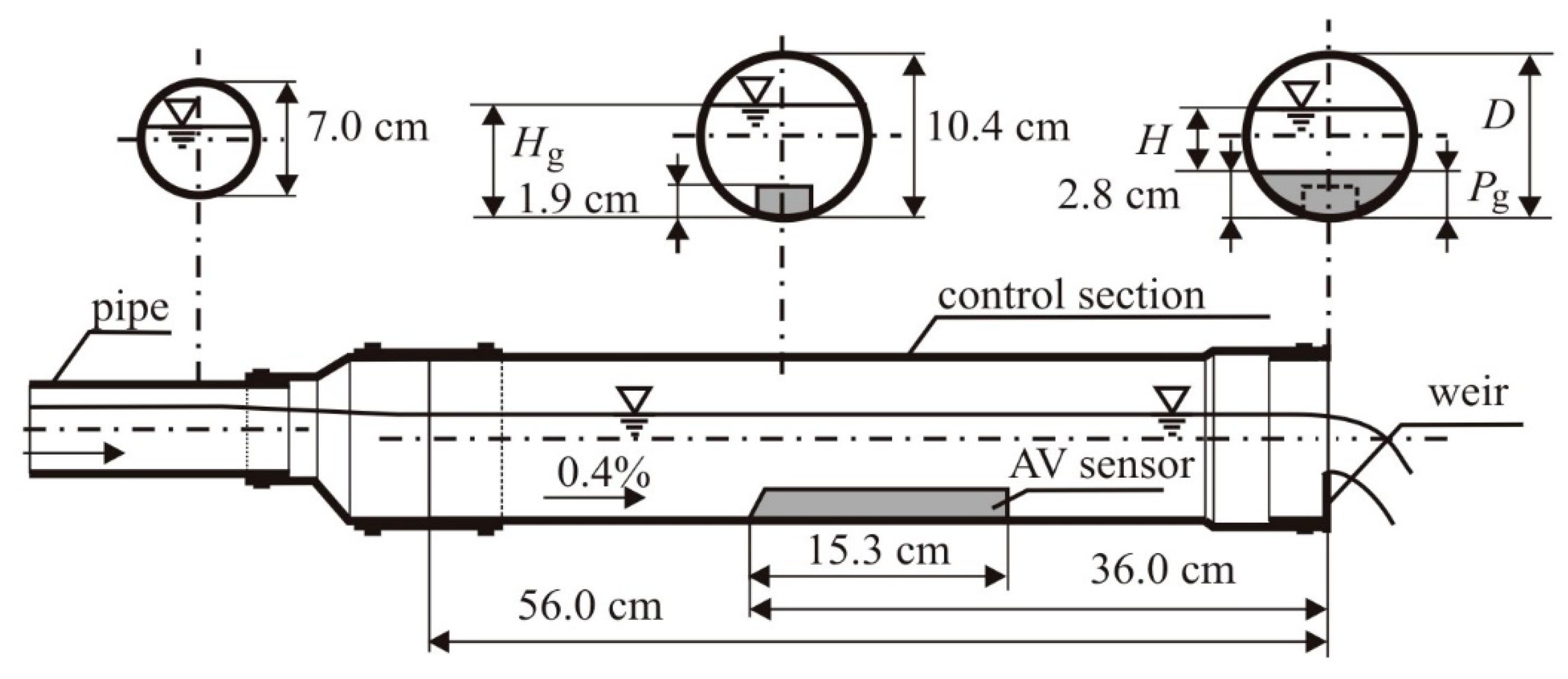
The experimental stand reflected field conditions prevailing in a drainage pipe. The problem with a drainage pipe is its relatively small diameter, low flow, and insufficient water level for AV measurements during some parts of the season. Previous research has shown that discharge measurements by a control section with the same diameter as a drainage pipe (75 mm) were characterized by poor accuracy, especially for zones of very low and high discharges [23]. Thus, an appropriate pipe was assembled, where the diameter and input of the outlet weir guaranteed the maintenance of minimum filling in the pipe measuring section. Because of the drain well dimensions, where area velocity had to work on purpose, as well as the AV sensor requirements, the control section with the outlet weir had a larger diameter than the drainage pipe. The AV sensor was installed in a polypropylene pipe (control section) with a diameter of 104 mm and a length of 560 mm [24]. The control section with an AV sensor inside is presented in Scheme 1. The submergence of the AV sensor provided an outlet weir with height (Pg), according to Scheme 1 and Scheme 2a or high water level on the outflow simulated in laboratory conditions with an adjustable weir located at the end of the experimental stand (Scheme 2b,c).
The control section was constructed in such a way that it could be easily moved and installed into a drainage well in the field after disconnection from the experimental site. Using the same control section for laboratory tests and field measurements guarantees the same measuring conditions for area velocity. In this way, installation errors that could affect the measurement characteristics were avoided. The values measured with the area velocity were correlated with the values obtained from the reference method. A parallel set of AV and REF data gave a simultaneous determination of the flow rate. The area velocity enabled the determination of water levels in the pipe, average flow rate, and flow velocity, as well as water temperature. The laboratory system with an electromagnetic flow meter (REF) enabled flow rate and water level control in the supply pipe and water temperature measurement in the system tank. The AV meter measured the water level in the pipeline and the average flow velocity and determined the flow calculated from the product of this velocity and the area of the cross section of the stream. To determine the hydraulic conditions of the device’s operation, the values of the flow velocity were used because this is the quantity according to which the critical water movement and types of water movement (supercritical or subcritical) are defined. Velocity values were interpreted according to the flow phases that can occur in such an extended section of the pipe. Typically, these analyses use flow velocity not total flow rate. The REF and AV devices measure hydraulic quantities regardless of the pipeline geometry and flow conditions in the device. Therefore, they are universal in nature and widely used in hydraulic measurements (REF in laboratory and AV in field tests).
In order to identify the values, indices were introduced: AV for area velocity-related values and REF for laboratory flow meter-related values (for example, VAV, VREF). The measurements of water level, average flow velocity, and average flow rate were conducted in steady, identical 15 s intervals for both flow meters. The determination of the pipe submergence’s influence on its discharge required checking AV behavior in the possible modelling and variable measuring conditions occurring at the end of the drainage pipe in the field. The investigations reproduced variable flow conditions in a drainage pipe typical of drainage pipe systems during spring melting and sudden, intensive summer rains. Our research aimed to model the influence of possible high water level outflow on pipe cross-section flow capacity. The discharge simulation was performed due to the groundwater raising Q = f (T) for a constant level of lower water Hd. Depending on the submergence conditions of the outflow weir Pg and the fulfilment of the control section Hg, three flow phases with different hydraulic calculation roles were defined:
3. Results and Discussion
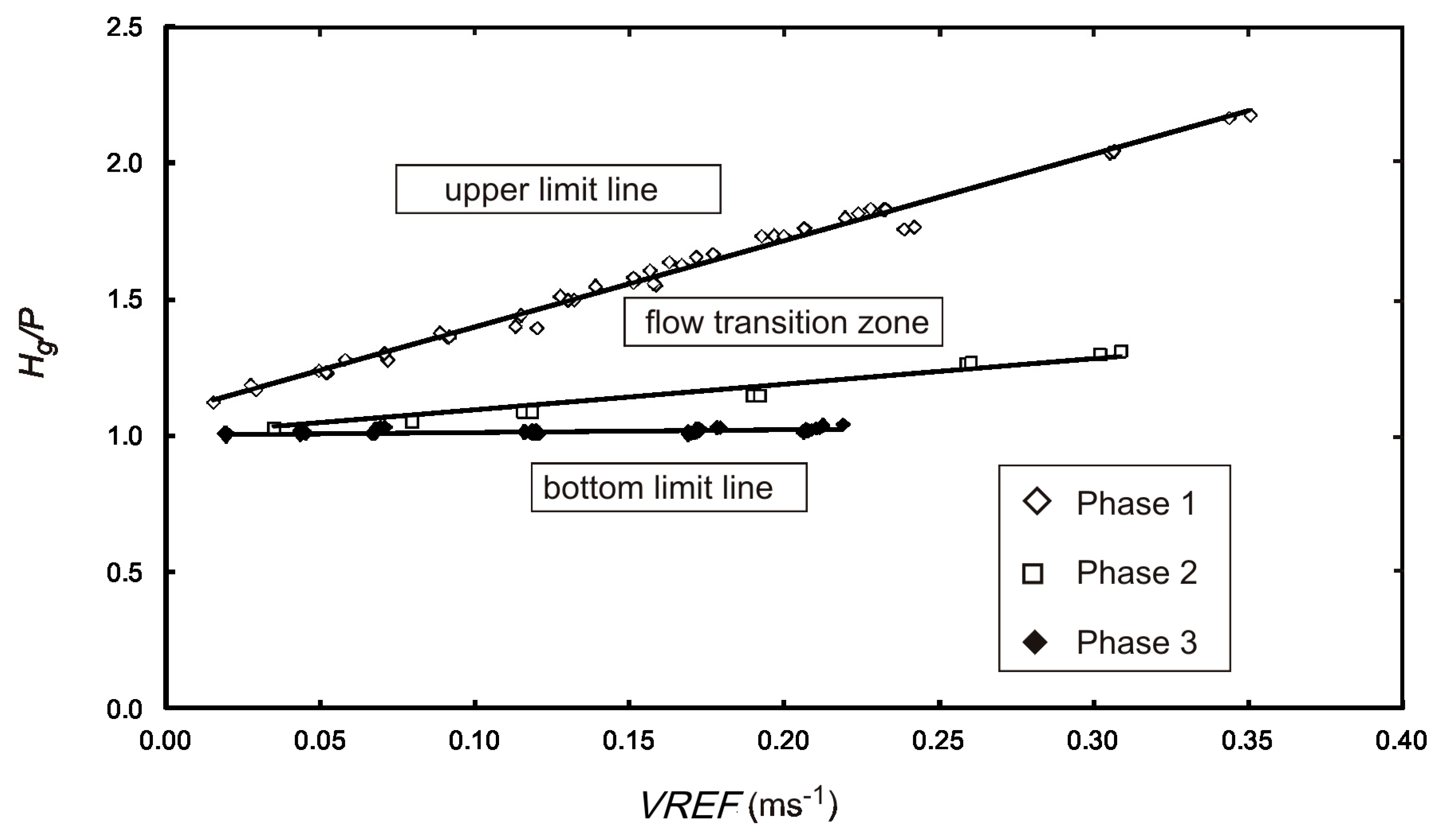
Because a control section has different hydraulic conditions compared to the recommended pipe for area velocity, the water level and flow velocity measured by area velocity required the determination of calibration curves or the elaboration of formulas, which enabled the measurement of values with respect to the reference values. Previous research [23,25] has proven a good agreement between control section water levels measured by AV and REF values. A differential pressure transducer of an AV probe is characterized by good accuracy and precision of measurement. However, there is an essential variance between the measured AV velocity values and the reference values controlled by a laboratory system. The diameter of the measuring (pipe) section and minimum water level determined by the outlet weir are the parameters which have the greatest impact. Another significant problem includes the variable hydraulic conditions in the drainage pipe system flow: The transition from a partially filled up drain with no pressure through a completely filled up drain still without pressure to a completely filled up drain pipe working with pressure. Assuming these three flow phases, velocity average values VREF related to dimensionless pipe filling (Hg/P) were elaborated (Figure 1). The calculated average values of VREF flow related to dimensionless pipe filling (Hg/P) formed three lines arranged in a circular fashion. The P value equalled the Pg value for the free flow phase, otherwise it was equal to the Hd value. The presented graph shows the three flow phases defined earlier. The upper limit line reflected Phase I flow conditions (Scheme 2a). A flow transition zone is placed between the limit lines. Points situated in this area represent the change of the free flow form with the outflow weir submergence to pressure flow (Scheme 2b). Points representing transient flow (Phase II) gather along lines within the considered zone. The position of these lines depends on the submergence of the weir. Points marked as Phase 2 (Figure 1) were obtained for Hd = 0.5D. The bottom limit line was determined using pipe pressured flow values (Scheme 2c).
Points marked as Phase 3 obtained for all examined low water levels gather around this line. The limitation of the lower water level Hd has no influence on the pipeline flow velocity. The assumption of flow velocity in a pipe as an analyzing measurement parameter is reasonable because the “Area-Velocity” flow meter option was applied in the software and the discharge was calculated according to average flow velocity (the AV software also has different options of discharge calculation, for example, Manning formula or two-term polynomial equations) [26]. Thus, the aim of the further analysis was the determination of the actual flow velocity in the control section. It was assumed that the actual velocity was equal to the velocity measured by the laboratory flow meter (VREF) and the independent variable was the velocity measured by area velocity (VAV). The relationship between the actual and the measured velocity values is presented in Figure 2.
The values of velocity measured by the AV method were higher than the expected values for each flow phase in each case. Fitting was done using linear regression y = ax. Considerable point scattering for free and transient flow could be observed, especially over VAV = 0.5 m s−1 (Figure 2a,b). The most accurate fitting was obtained for the pressured flow (R2 = 0.987), where the actual velocity VREF was equal to 0.428 of the measured velocity VAV (Figure 2c). The transient flow phase was relatively short because the rapid increase of lower water level Hd limited the possibility of outflow, leading to pressured flow (Phase III). Thus, a limited number of Phase II measured values gave rise to an unsatisfying fitting (R2 = 0.48). The flow Phase I (Figure 2a), as well as all the phases of flow (Figure 2d) fittings, gave similar results. The actual velocity VREF amounted to 0.508 and 0.849 of the measured velocity VAV, respectively (R2 = 0.85). From the practical point of view, it is difficult to watch for different outflow phases (especially Phase II) in a drainage pipeline. However, the most frequent flow case in a drainage pipeline is free flow. As proven above, the measured velocity VAV over 0.5 m s−1 was characterized by a significant instability. Thus, the calculated discharge values QAV would be inaccurate. Further research was focused on the correlation between the discharge calculated by the chosen formula and the reference discharge QREF. The discharge along the control section (Scheme 1), working in the free outflow conditions (Scheme 2a, Phase I) can be determined according to the well-known Cipolletti formula [27,28]:
where B is the crest length of the weir (equals to 0.0895) (m), g is the acceleration of gravity (m s−2), H is the water level over the weir head (cm), and μ is the flow rate coefficient calculated by the following equation:
Another method of discharge calculation is the California pipe method adapted to the measurement of comparatively small flows in pipes. The empirically developed rating formula for the California pipe method is as follows [22]:
where h is the liquid level at the pipe outlet (m), and d is the pipe diameter (m).
The California pipe method was originally designed for the free pipe outflow conditions [22]. The idea of this research was to adopt the California pipe method for the calculation of free flow outlet weir discharge (Scheme 2a, Phase I). For this purpose, exponents of Equation (3) had to be optimized. The optimization was conducted on the basis of QREF values related to water level over weir head H using the non-linear regression method. As a result, the following form of the California pipe method was devised (called the California pipe outlet weir method—Cpw for contradistinction):
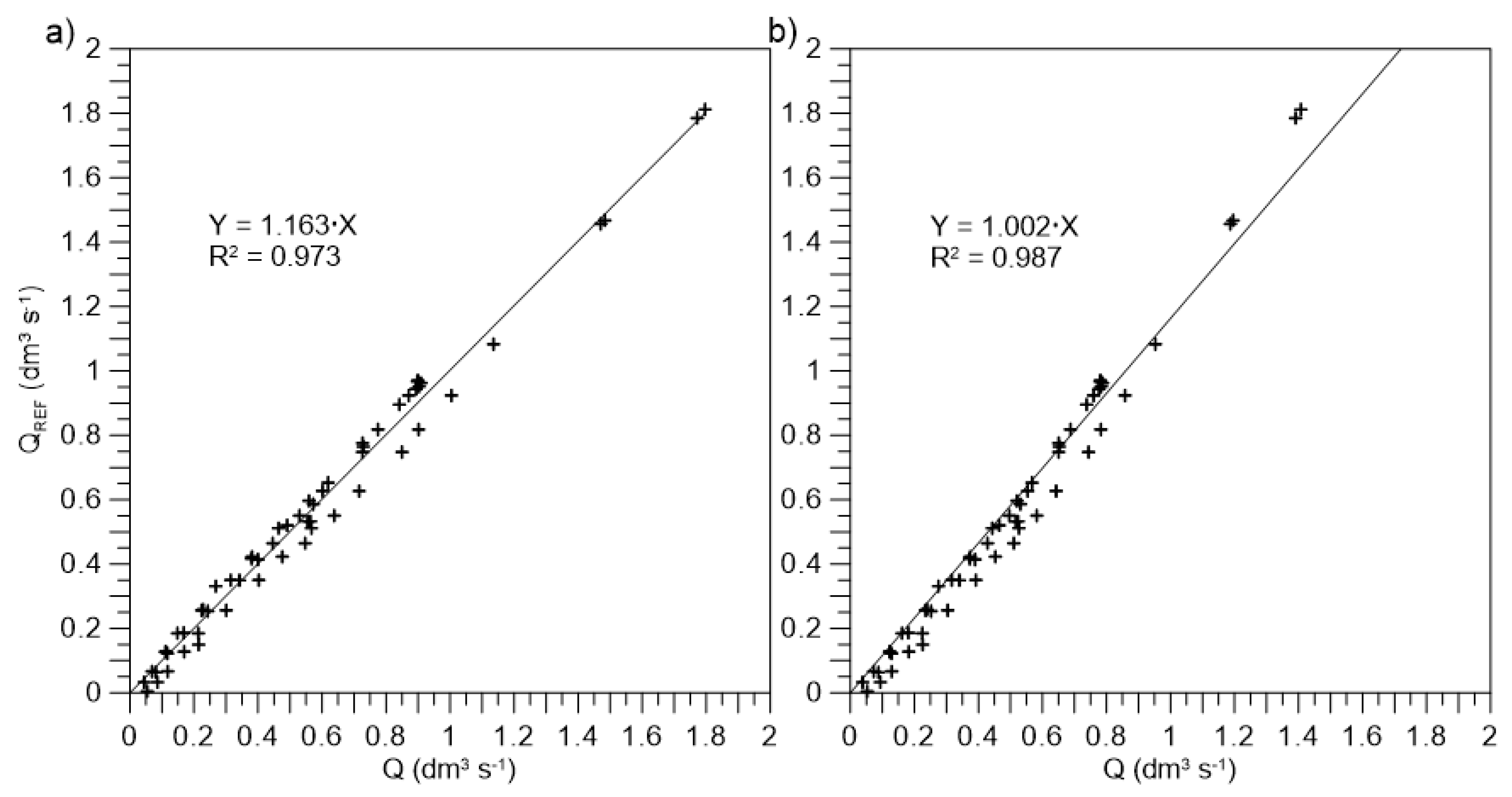
The relationship between the measured (QREF) and the discharge values calculated using Equations (1) and (4) is presented in Figure 3. For an accurate evaluation of the considered relationship, the following statistical criteria were applied: The maximum error value (ME), the root-mean-square error value (RMSE), the coefficient of determination value (CD), and the coefficient of residual mass value (CRM) [29]. The ME value is the maximum difference between the observed and the calculated value and indicates the worst case calculated by equation. The RMSE value indicates to what extent the calculations are over- or underestimating the measurements, expressed as a percentage of the averaged value of the measurements. The CD describes the ratio between the scattering of the calculated values and the scattering of the measurements. The CD value proves the dynamics in the measured and calculated values’ agreement.
The CRM value indicates whether the calculations tend to overestimate or to underestimate the measurements. A negative CRM value indicates a tendency to overestimate. Statistical results are presented in Table 1.
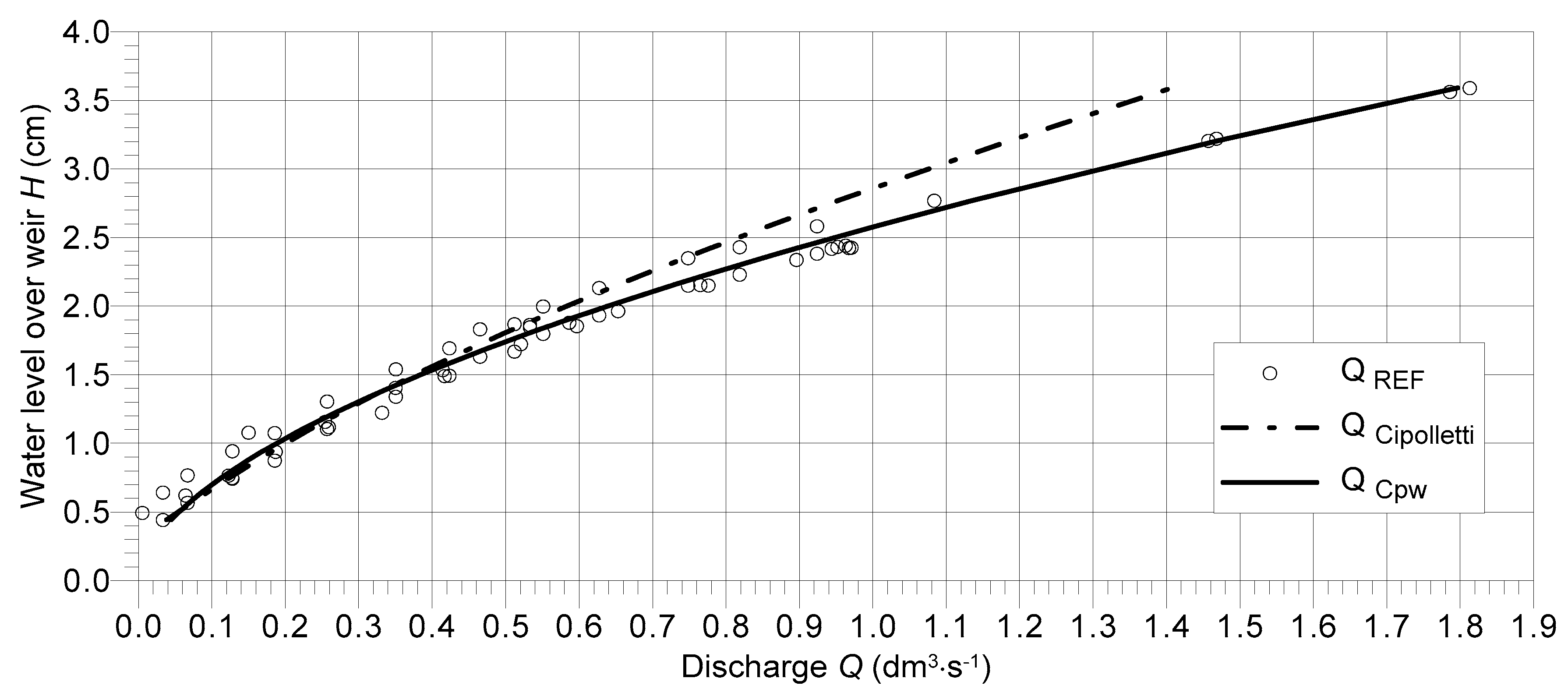
All the specified statistics proved that the best results were obtained for the values calculated by the California pipe outlet weir method (Figure 3b). It can be assumed that the discharge values calculated with this method were very close to the measured (reference) values. The worst results were given by the Cipolletti equation. Thus, the obtained results were underestimated by about 16% in relation to the reference discharge values (Figure 3a). Discharge curves calculated by Equations (1) and (4), as well as measuring points, are presented in Figure 4. It can be noted that the most appropriate equation for the calculation of the discharge free flow case was the California pipe outlet weir method. The Cipolletti formula is not recommended for the calculation of discharge in the considered case.
4. Conclusions
Previous research proved to be in good agreement with the control section water level measured by area velocity flow meter and the reference values measured by the laboratory method. Thus, the values obtained with the AV method are characterized by good accuracy and they can be used for the calculation of discharge.
There is an essential variance between the velocity values measured by ultrasonic flow meter and the reference values controlled by the laboratory method. Differences result from the specific measurement conditions, which appear in the drainage pipe system. The relatively small diameter of the measuring pipe section and the minimum water level determined by the outlet weir were the factors having the greatest influence. Another significant problem concerning the flow velocity measurement was the variable hydraulic conditions in the drainage pipe system flow: The transition from a partially filled up drain with no pressure through a completely filled up drain still without pressure to a completely filled up drain pipe working over pressure.
The values of velocity measured by the ultrasonic flow meter were higher than the reference values for each flow phase. The best relationship between the measured and the reference velocity values was obtained for the pressured flow, where the expected velocity was equal to 0.428 of the measured velocity. The measured velocity for the three aforementioned conditions was characterized by significant variability in relation to the reference velocity. Thus, the calculated discharge based on the measured velocity of the ultrasonic flow meter could be responsible for a substantial error.
The best results of the calculated discharge were obtained by means of an elaborated method named the California pipe outlet weir method (adapting the California pipe method for this purpose). The discharge values calculated with this method were very close to the reference values.
The discharge from a tile drain working on a partially filled up pipe with no pressure should be calculated using the California pipe outlet weir method, whereas the discharge from a completely filled up drain pipe working over pressure should be calculated as the ratio between 0.428 times the measured velocity and the pipe cross-section area.
Author Contributions
Conceptualization, D.S., S.B.; Methodology, D.S., S.B.; Formal analysis, D.S., S.B.; Investigation, D.S., S.B.; Resources, D.S.; Data Curation, D.S., S.B.; Writing—Original Draft Preparation, D.S., S.B.; Writing—Review & Editing, D.S.; Visualization, D.S., S.B., Supervision, D.S.; Project Administration, D.S.; Funding Acquisition, D.S.
Funding
This research was founded by the Polish Ministry of Science and Higher Education, grant Nos. N N305 039234 and N N305 171840.
Acknowledgments
Special thanks to Eng. Zygmunt Pietraszek for his invaluable help in conducting laboratory tests.
Conflicts of Interest
The authors declare no conflict of interest.
References
- De Schepper, G.; Therrien, R.; Refsgaard, J.C.; Hansen, A.L. Simulating coupled surface and subsurface water flow in a tile-drained agricultural catchment. J. Hydrol. 2015, 521, 374–388. [Google Scholar] [CrossRef]
- Kladivko, E.J.; Willoughby, G.L.; Santini, J.B. Corn Growth and Yield Response to Subsurface Drain Spacing on Clermont Silt Loam Soil. Agron. J. 2005, 97, 1419–1428. [Google Scholar] [CrossRef] [Green Version]
- Szejba, D.; Cymes, I.; Szatyłowicz, J.; Szymczyk, S. An impact of drainage system on soil water conditions at Lidzbark Warmiński experimental site. Biologia 2009, 64, 565–569. [Google Scholar] [CrossRef]
- Šimůnek, J.; Jarvis, N.J.; van Genuchten, M.Th.; Gärdenäs, A. Review and comparison of models for describing non-equilibrium and preferential flow and transport in the vadose zone. J. Hydrol. 2003, 272, 14–35. [Google Scholar] [CrossRef]
- de Ridder, N.A.; Boonstra, J. Analysis of Water Balances. In Drainage Principles and Application; Ritzema, H.P., Ed.; International Institute for Land Reclamation and Improvement Publication 16. Second Edition; International Institute for Land Reclamation and Improvement/ILRI: Wageningen, The Netherlands, 1994; pp. 601–633. ISBN 90-70754-3-39. [Google Scholar]
- Skaggs, R.W. Drainmod. Methods for Design and Evaluation of Drainage—Water Management Systems for Soils with High Water Tables; Reference Report; USDA-SCS, South National Technical Center: Fort Worth, TX, USA, 1989. [Google Scholar]
- Hansen, A.L.; Refsgaard, J.C.; Christensen, B.S.B.; Jensen, K.H. Importance of including small-scale tile drain discharge in the calibration of a coupled groundwater-surface water catchment model. Water Resour. Res. 2013, 49, 585–603. [Google Scholar] [CrossRef] [Green Version]
- Arnold, J.G.; Srinivasan, R.; Muttiah, R.S.; Williams, J.R. Large area hydrologic modeling and assessment part I: Model development. J. Am. Water Resour. Assoc. 1998, 34, 73–89. [Google Scholar] [CrossRef]
- Bauwe, A.; Kahle, P.; Lennartz, B. Hydrologic evaluation of the curve number and Green and Ampt infiltration methods by applying Hooghoudt and Kirkham tile drain equations using SWAT. J. Hydrol. 2016, 537, 311–321. [Google Scholar] [CrossRef]
- Kiesel, J.; Fohrer, N.; Schmalz, B.; White, M.J. Incorporating landscape depressions and tile drainages of a northern German lowland catchment into a semi-distributed model. Hydrol. Process. 2010, 24, 1472–1486. [Google Scholar] [CrossRef]
- Koch, S.; Bauwe, A.; Lennartz, B. Application of the SWAT model for a tile-drained lowland catchment in North-Eastern Germany on subbasin scale. Water Resour. Manag. 2013, 27, 791–805. [Google Scholar] [CrossRef]
- Szejba, D. Wykorzystanie modelu SWAP do oceny elementów bilansu wodnego gleby pyłowej. Zesz. Probl. Postęp. Nauk Rol. 2001, 477, 177–186. [Google Scholar]
- Szejba, D.; Brandyk, T. Zastosowanie modelu SWAP do prognozowania elementów bilansu wodnego zdrenowanej gleby pyłowej. Zesz. Probl. Postęp. Nauk Rol. 2005, 506, 461–469. [Google Scholar]
- van Dam, J.C.; Huygen, J.; Wesseling, J.G.; Feddes, R.A.; Kabat, P.; van Walsum, P.E.V.; Groenendijk, P.; van Diepen, C.A. Theory of SWAP Version 2.0; Technical Document 45; DLO Winand Staring Centre: Wageningen, The Netherlands, 1997; pp. 19–48. [Google Scholar]
- Khan, A.H.; Ong, C.K. Design and calibration of tipping bucket system for field quantification. J. Soil Water Conserv. 1997, 52, 437–443. [Google Scholar]
- Enamorado, S.M.; Hurtado, M.D.; Andreu, L.; Martinez, F.; Sanchez, J.; Delgado, A.; Abril, J.M. Development of a recording water flow meter using ultrasonic measurement of water levels in a slotted U-pipe. Agric. Water Manag. 2007, 88, 263–268. [Google Scholar] [CrossRef]
- Maheepala, U.K.; Takyi, A.K.; Perera, B.J.C. Hydrological data monitoring for urban stromwater drainage systems. J. Hydrol. 2001, 245, 32–47. [Google Scholar] [CrossRef]
- Unidata Australia. User Manual for STARFLOW Ultrasonic Doppler Instrument with MicroLogger, Revision-D; Unidata Australia: Willetton, Australia, 1996. [Google Scholar]
- Teledyne ISCO. 2150 Area Velocity Flow Module and Sensor. Installation and Operation Guide; Teledyne ISCO, Incl.: Lincoln, NE, USA, 2008. [Google Scholar]
- Akgiray, Ö. Simple Formulae for Velocity, Depth of Flow, and Slope Calculations in Partially Filled Circular Pipes. Environ. Eng. Sci. 2004, 21, 371–385. [Google Scholar] [CrossRef]
- Erb, H.G. Technika Pomiarów Przepływu Wody i Ścieków; Seidel-Przywecki: Szczecin, Poland, 1999; pp. 150–192. ISBN 83-910801-0-2. [Google Scholar]
- Walkowiak, D.K. ISCO Open Channel Flow Measurement Handbook, 6th ed.; Teledyne ISCO, Incl.: Lincoln, NE, USA, 2008; pp. 132–142. ISBN 0-9622757-3-5. [Google Scholar]
- Szejba, D.; Bajkowski, S.; Pietraszek, Z. Możliwości wykorzystania ultradźwiękowych mierników do pomiaru przepływu w rurociągach drenarskich. In Hydrologia w Inżynierii i Gospodarce Wodnej: Tom 1; Więzik, B., Ed.; Monografie Komitetu Inżynierii Środowiska PAN: Warszawa, Poland, 2010; Volume 68, pp. 439–449. ISBN 978-83-89293-93-0. [Google Scholar]
- Bajkowski, S.; Szejba, D. Adapter for Measuring Water Flow in Pipes. Patent Number PL396437-A1, 2015. [Google Scholar]
- Popek, Z.; Hejduk, L.; Hładki, P. Możliwości wykorzystania przepływomierza modułowego ISCO 2150 w pomiarach hydrometrycznych w małej rzece nizinnej. Sci. Rev. Eng. Env. Sci. 2011, 53, 247–257. [Google Scholar]
- Teledyne ISCO. Flowlink 5 Software Instruction Manual; Teledyne ISCO, Incl.: Lincoln, NE, USA, 2005. [Google Scholar]
- Dąbkowski, L.; Skibiński, J.; Żbikowski, A. Hydrauliczne Podstawy Projektów Wodno-Melioracyjnych; PWRiL: Warszawa, Poland, 1982; pp. 161–242. ISBN 83-09-00407-9. [Google Scholar]
- Hively, W.D.; McCarty, G.W.; Angier, J.T.; Geohring, L.D. Weir Design and Calibration for Stream Monitoring in a Riparian Wetland. Hydrol. Sci. Technol. 2006, 22, 71–82. [Google Scholar]
- Loague, K.; Green, R.E. Statistical and graphical methods for evaluating solute transport models. Overview and application. J. Contam. Hydrol. 1991, 7, 51–73. [Google Scholar] [CrossRef]
Scheme 1.
Control section with an area velocity ultrasonic flow meter (AV) sensor inside, where D is the pipe diameter, Pg is the outlet weir height, and Hg is the control section water level [24].
Scheme 1.
Control section with an area velocity ultrasonic flow meter (AV) sensor inside, where D is the pipe diameter, Pg is the outlet weir height, and Hg is the control section water level [24].

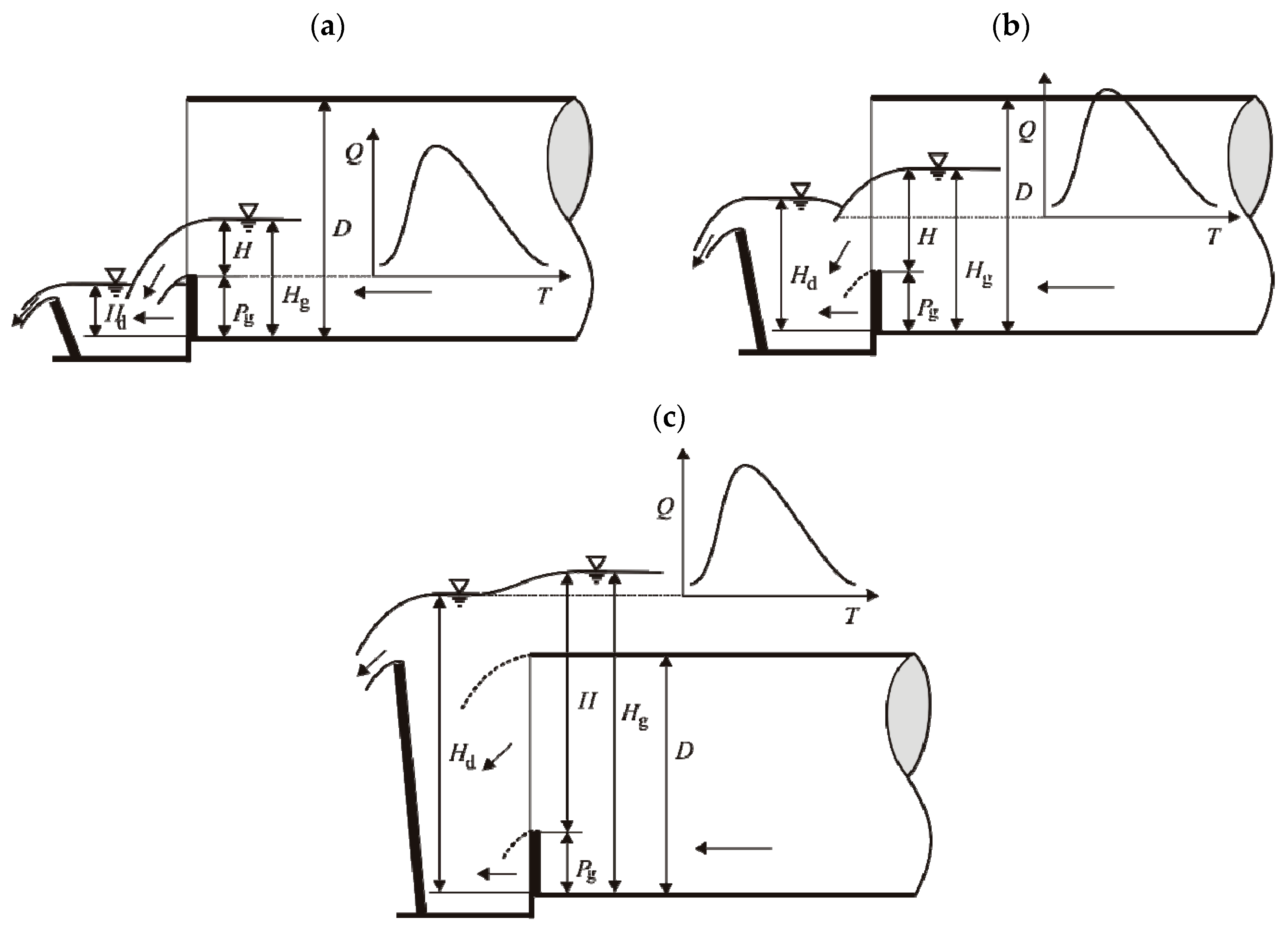
Scheme 2.
Unsubmerged weir and unpressured pipe (a); submerged weir and unpressured pipe (b); submerged weir and pressured pipe (c); Q is the discharge (dm3 s−1), T is time (s), H is the water level above the weir (mm), and Hd is the lower water level (mm).
Scheme 2.
Unsubmerged weir and unpressured pipe (a); submerged weir and unpressured pipe (b); submerged weir and pressured pipe (c); Q is the discharge (dm3 s−1), T is time (s), H is the water level above the weir (mm), and Hd is the lower water level (mm).

Figure 1.
Velocity average values VREF related to dimensionless pipe filling Hg/P: Phase 1 is free flow, Phase 2 is transient flow, and Phase 3 is pressured flow.
Figure 1.
Velocity average values VREF related to dimensionless pipe filling Hg/P: Phase 1 is free flow, Phase 2 is transient flow, and Phase 3 is pressured flow.

Figure 2.
Relationship between the real velocity VREF and the measured VAV for free flow (a), transient flow (b), pressured flow (c), and all phases of flow together (d).
Figure 2.
Relationship between the real velocity VREF and the measured VAV for free flow (a), transient flow (b), pressured flow (c), and all phases of flow together (d).

Figure 3.
Relationship between the measured discharge QREF and the calculated Q by Equation 1 (a) and Equation 4 (b).
Figure 3.
Relationship between the measured discharge QREF and the calculated Q by Equation 1 (a) and Equation 4 (b).

Figure 4.
Relationship between the discharge and the water level over the weir.


Table 1.
Description of statistical criteria values for measured and calculated discharge. ME: maximum error, RMSE: root-mean-square error, CD: coefficient of determination, CRM: residual mass
Table 1.
Description of statistical criteria values for measured and calculated discharge. ME: maximum error, RMSE: root-mean-square error, CD: coefficient of determination, CRM: residual mass
| Statistical Criteria | Equation (1) | Equation (4) | |
|---|---|---|---|
| ME (dm3 s−1) | range: (0; ∞) best value: 0 | 0.406 | 0.101 |
| RMSE (%) | range: (−∞; ∞) best value: 0 | 21.12 | 8.24 |
| CD (-) | range: (0; ∞) best value: 1 | 1.600 | 1.028 |
| CRM (-) | range: (−∞; ∞) best value: 0 | −0.105 | 0 |
© 2019 by the authors. Licensee MDPI, Basel, Switzerland. This article is an open access article distributed under the terms and conditions of the Creative Commons Attribution (CC BY) license (http://creativecommons.org/licenses/by/4.0/).
Share and Cite
MDPI and ACS Style
Szejba, D.; Bajkowski, S. Determination of Tile Drain Discharge under Variable Hydraulic Conditions. Water 2019, 11, 120. https://doi.org/10.3390/w11010120
AMA Style
Szejba D, Bajkowski S. Determination of Tile Drain Discharge under Variable Hydraulic Conditions. Water. 2019; 11(1):120. https://doi.org/10.3390/w11010120
Chicago/Turabian StyleSzejba, Daniel, and Sławomir Bajkowski. 2019. "Determination of Tile Drain Discharge under Variable Hydraulic Conditions" Water 11, no. 1: 120. https://doi.org/10.3390/w11010120
Note that from the first issue of 2016, this journal uses article numbers instead of page numbers. See further details here.