Evaluation of Hydrological Application of CMADS in Jinhua River Basin, China

Abstract

Evaluating the hydrological application of reanalysis datasets is of practical importance for the design of water resources management and flood controlling facilities in regions with sparse meteorological data. This paper compared a new reanalysis dataset named CMADS with gauge observations and investigated the performance of the hydrological application of CMADS on daily streamflow, evapotranspiration, and soil moisture content simulations. The results show that: CMADS can represent meteorological elements including precipitation, temperature, relative humidity, and wind speed reasonably for both daily and monthly temporal scales while underestimates precipitation compared with gauge observations slightly (<15%). The hydrological model using CMADS dataset as meteorological inputs can capture the daily streamflow chracteristics well overall (with a NS value of 0.56 during calibration period and 0.61 during validation period) but underestimates streamflow obviously (with a BIAS of $-42.42$% during calibration period and a BIAS of $-33.29$% during validation period). The underestimation of streamflow simulated with CMADS dataset is more seriously in dry seasons ($-48.40$%) than that in wet seasons ($-39.41$%) for calibration period. The model driven by CMADS estimates evapotranspiration and soil moisture content well compared with the model driven by gauge observations.

1. Introduction

The magnitude and frequency of floods and droughts, companied with substantially social and economic losses, are increasing with global warming in many regions around the world [1,2,3]. Hydrological simulations are the major tool of water resource management for forecasting floods and droughts [4,5,6]. With the development of hydrological science and computing science, some complicated physically-based spatial distributed hydrological models have been developed [7,8]. These models are able to simulate the types, intensities, and locations of runoff production through considering complicated interactions of topography, soil characteristics, vegetation, and climate [9,10,11]. However, they have higher requirements in the spatiotemporal resolution of meteorological inputs [12]. Meteorological data such as precipitation, temperature, and wind speed are usually observed and collected using gauges and meteorological radar networks. These meteorological devices are usually deployed sparsely in some regions because of topographical and economical limitations, and thus, inadequate to meet the requirements of complicated distributed hydrological models [13].

In recent decades, reanalysis datasets with relatively high spatiotemporal resolution are developed as complementation of gauge observations in data sparse areas [14]. They combine numerical weather prediction (NWP) model and satellite-based products and/or gauge observations by data assimilation technologies. Reanalysis datasets usually have long time series and contain most types of meteorological elements needed by hydrological models and have been used in many different sectors. For example, Sheffield et al. [15] created a global dataset of meteorological forcings by combining the National Centers for Environmental Prediction-National Center for Atmospheric Research reanalysis (NCEP-NCAR) with a suite of global observation-based dataset. The dataset can be used to drive land surface hydrological models. Tang et al. [16] assessed the historical trend of Antarctic precipitation and temperature using reanalysis datasets including the European Centre for Medium-range Weather Forecasts “Interim” reanalysis (ERA-Interim), the National Centers for Environmental Prediction Climate Forecast System Reanalysis (CFSR), the Japan Meteorological Agency 55-year Reanalysis (JRA-55), and the Modern Era Retrospective-analysis for Research and Applications (MERRA). Maurer et al. [17] reproduced and analyzed the hydrologic budgets over the Mississippi River basin using the National Centers for Environmental Prediction (NCEP)/National Center for Atmospheric Research (NCAR) reanalysis (NRA1) and the follow-up NCEP/Department of Energy (DOE) reanalysis (NRA2). However, errors and uncertainties may be attributed to shortcomings associate with NWP model structures, data assimilation methods, and source data used to assimilation [18,19]. Some previous studies have shown that newer reanalysis datasets perform better than older datasets in identifying recurrent extratropical cyclones [20], in capturing daily variability of precipitation [21], and some other meteorological elements [22] because of improvements in observation system, model structure, and data assimilation method. Dee et al. [22] pointed out that the initialization of an NWP model that has a significant effect on the quality of reanalysis data is determined by observed data. Moreover, the density, type, and quality of observed data are changing over time, which can introduce spurious errors into reanalysis datasets [23]. The China Meteorological Assimilation Driving Datasets for the SWAT model (CMADS) is a new reanalysis that focuses on East Asia areas and available online (www.cmads.org). It was developed by Dr. Xianyong Meng from the China Agricultural University (CAU) using STMAS assimilation techniques and big data projection and processing methods [24]. The dataset compensates for the shortcoming that few meteorological reanalysis were developed for East Asia particularly and has received attention all over the world [25,26,27,28,29,30,31,32]. The evaluation and hydrological application of CMADS have been performed in many regions such as the Juntanghu watershed [33], the Manas River basin [30], and the Qinghai-Tibet Plateau. Fubo Zhao et al. [25] analyzed the parameter uncertainty of the SWAT model in a mountain-loess transitional watershed on the Chinese Loess Plateau using CMADS dataset. Thom et al. [26] evaluated the performance of CMADS in streamflow simulation in Han River basin in the Korean Peninsula. However, most evaluations were focused on streamflow simulation and ignored other hydrological fluxes such as evapotranspiration. Because of the uncertainty of hydrological model, good performance in streamflow simulation may be based on bad performance in other hydrological fluxes. The purpose of this study is to identify whether CMADS is appropriate to the simulation of entirely hydrological processes including streamflow, evapotranspiration, and soil moisture. Besides, it is the first evaluation of CMADS in regions dominated by mold rain. The results can provide reference for the application of CMADS in regions dominated by mold rain.

The paper is organized as follows. Section 2 illustrates the materials and methods. Section 3 describes the evaluation results of CMADS dataset, and a further discussion is given in Section 4. Finally, a brief summary is given in Section 5.

2. Materials and Methodology

2.1. Study Area

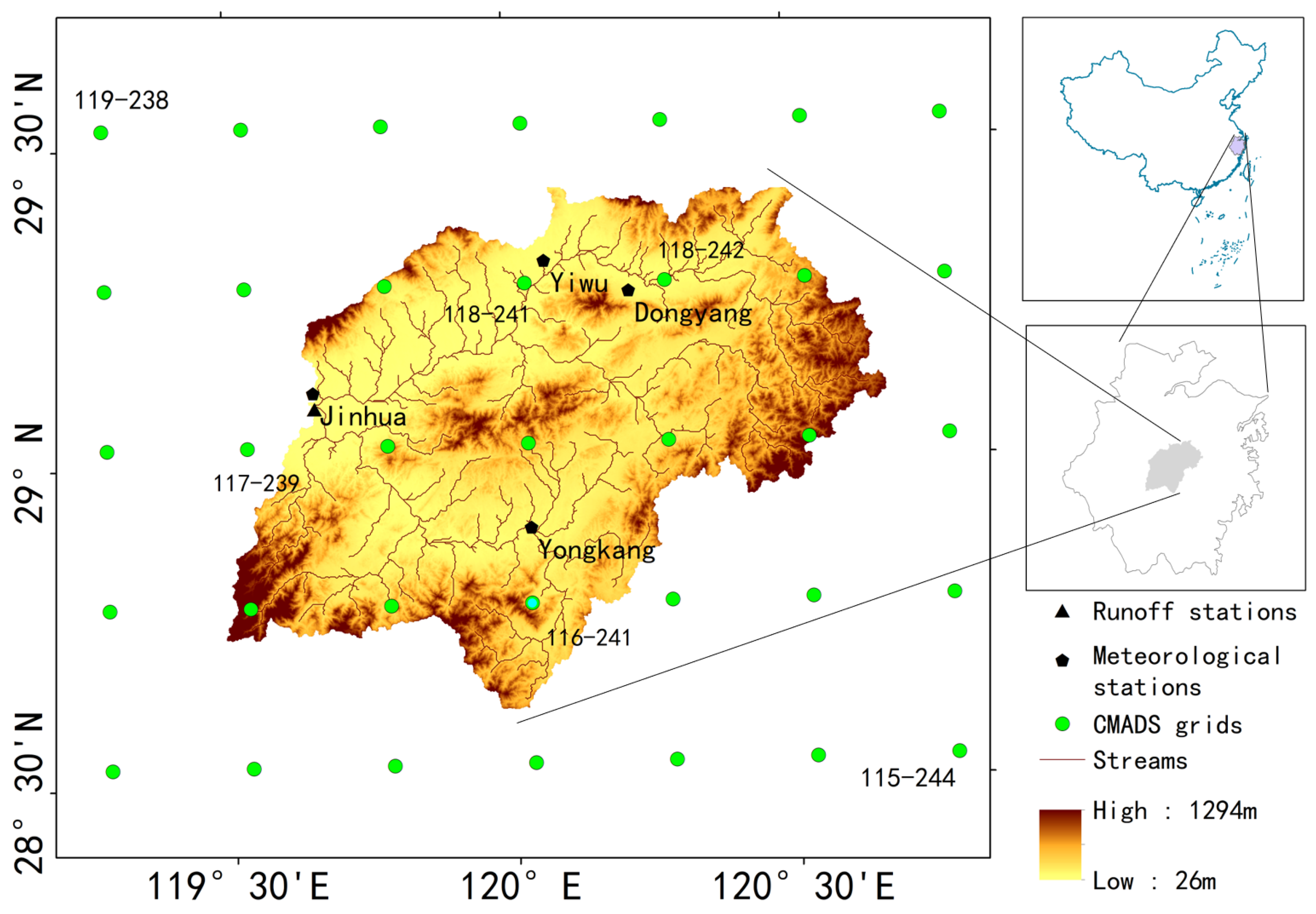
Jinhua River is a tributary of Qiantang River, the largest river in Zhejiang Province, East China. It is originated from Panan County, with a total length of 195 km. The drainage area of Jinhua River is about 6782 km${}^2$. This study focuses on the basin above Jinhua hydrological station whose drainage area is 5996 km${}^2$. The basin is dominated by humid monsoon. The mean annual precipitation of this basin is about 1500 mm. The climate of this basin is characterized by hot rainy summers and cold dry winters. The precipitation occurring during the period from May to July accounts for more than half of the annual total precipitation. The average temperature is ranging between 15–18 °C. The maximum annual temperature is about 40 °C. The basin elevation ranges from 20 to 1300 m (based on China National Height Datum). The main landuse types of this basin are agricultural land and forest and the main soil type is clay loam. For more information about the studied area, readers are referred to Xu et al. [34]. The location, elevation, hydrometeorological stations, and CMADS grids used in the study are shown in Figure 1.

2.2. Data

Daily values of average atmospheric temperature, wind speed, relative humidity, shortwave radiation, long wave radiation, and precipitation were used to drive the distributed hydrology-soil-vegetation model (DHSVM). Meteorological data from gauge observations and the CMADS were compared and used as meteorological inputs of DHSVM. CMADS does not provide long wave radiation. In this paper, we calculated the sunshine duration using the shortwave radiation and then calculated the long wave radiation using the calculated sunshine duration. Gauge observations derived from Jinhua, Yiwu, Yongkang, and Dongyang stations are obtained from China Meteorological Administration while the CMADS dataset is available on the internet (www.cmads.org). The spatial resolution of CMADS is 0.25° (28 km). Daily discharge at Jinhua hydrological station is obtained from hydrological yearbook of China. The time period of meteorological and runoff data used in this study is from 2008 to 2013.

The DHSVM model needs digital elevation model (DEM), landuse types, soil types, river networks, and so on. In this study, the 90 m DEM is downloaded from the website of the Shuttle Radar Topography Mission (SRTM) (http://srtm.csi.cgiar.org/). The river network is generated based on DEM. The 1 km landuse data are obtained from Global Land Cover 2000 (GLC2000) program (http://bioval.jrc.ec.europa.eu/products/glc2000/products.php) while soil types data with a resolution of 500 m are obtained from Nanjing Institute of Soil Research, China.

2.3. Straightforward Comparison

Estimates of precipitation, average temperature, wind speed and relative humidity derived from the CMADS were compared with gauge observations before used as inputs of hydrological model. Three comparison strategies were used: (1) Basin average values of CMADS dataset and gauge observations calculated through Theissen polygon method were compared; (2) In CMADS dataset, the value of a grid is seen as the average value of the square centered on this grid. the value between a gauge and the square where the gauge locate was compared; and (3) Gauge observations were firstly interpolated into the same grid scale as CMADS using inverse distance weighting (IDW) method and then compared with CMADS datasets for each grid. In the second strategy, CMADS grid 117–239, 118–241, 118–242, and 116–241 were compared with Jinhua, Yiwu, Dongyang, and Yongkang respectively (Figure 1). The third strategy was only used to evaluation precipitation because that precipitation is much more spatially sensitive than other meteorological factors. The comparisons of all the meteorological elements mentioned above were made for daily and monthly temporal scales.

Diagnostic Statistics

The correlation coefficient (CC), the mean error (ME), the root mean squared error (RMSE), and the relative bias (BIAS) were used to evaluate the CMADS estimates including average temperature, wind speed, relative humidity, and precipitation for daily and monthly timesteps. Moreover, three other statistic indexes were calculated for daily precipitation. They are the probability of detection (POD), the false alarm ratio (FAR), and the critical success index (CSI). In the evaluation, the days when precipitation is >1 mm are considered as wet days [35]. The description of these symbols refers to Gao et al. [36]. The mathematical expressions of these indexes are the following [11,37]:

$$\mathit{C}\mathit{C}=\frac{{\sum }_{\mathit{i}=\mathbf{1}}^{\mathit{n}}({\mathit{G}}_{\mathit{i}}-\overline{\mathit{G}})({\mathit{S}}_{\mathit{i}}-\overline{\mathit{S}})}{\sqrt{{\sum }_{\mathit{i}=\mathbf{1}}^{\mathit{n}}{({\mathit{G}}_{\mathit{i}}-\overline{\mathit{G}})}^{\mathbf{2}}}\sqrt{{\sum }_{\mathit{i}=\mathbf{1}}^{\mathit{n}}{({\mathit{S}}_{\mathit{i}}-\overline{\mathit{S}})}^{\mathbf{2}}}}$$

(1)

$$\mathit{M}\mathit{E}=\frac{\mathbf{1}}{\mathit{n}}\sum _{\mathit{i}=\mathbf{1}}^{\mathit{n}}({\mathit{S}}_{\mathit{i}}-{\mathit{G}}_{\mathit{i}})$$

(2)

$$\mathit{R}\mathit{M}\mathit{S}\mathit{E}=\sqrt{\frac{\mathbf{1}}{\mathit{n}}\sum _{\mathit{i}=\mathbf{1}}^{\mathit{n}}{({\mathit{S}}_{\mathit{i}}-{\mathit{G}}_{\mathit{i}})}^{\mathbf{2}}}$$

(3)

$$\mathit{B}\mathit{I}\mathit{A}\mathit{S}=\frac{{\sum }_{\mathit{i}=\mathbf{1}}^{\mathit{n}}({\mathit{S}}_{\mathit{i}}-{\mathit{G}}_{\mathit{i}})}{{\sum }_{\mathit{i}=\mathbf{1}}^{\mathit{n}}{\mathit{G}}_{\mathit{i}}}\times \mathbf{100}\%$$

(4)

$$\mathit{P}\mathit{O}\mathit{D}=\frac{\mathit{H}}{\mathit{H}+\mathit{M}}$$

(5)

$$\mathit{F}\mathit{A}\mathit{R}=\frac{\mathit{F}}{\mathit{H}+\mathit{F}}$$

(6)

$$\mathit{C}\mathit{S}\mathit{I}=\frac{\mathit{H}}{\mathit{H}+\mathit{M}+\mathit{F}}$$

(7)

where $G_i$ represents gauge observations, $S_i$ is the CMADS estimates; H represents the observed daily precipitation that is correctly detected by CMADS; M represents the observed daily precipitation that is not detected by CMADS; F represents the daily precipitation that is detected by CMADS but not observed.

$CC$, ranging from $-1$ to 1, reflects the degree of linear correlation. Its best value is 1. ME reflects the average difference between the CMADS estimates and gauge observation with a range of $\left[0,+\infty \right)$. Its best value is 0. RMSE reflects the average error between the CMADS estimates and gauge observations with a range of $\left[0,+\infty \right)$. Its best value is 0. BIAS reflects the relative degree of the systematic error of the CMADS estimates with a range of $\left[0,+\infty \right)$. Its best value is 0. $POD$ is the fraction of rain occurrences that are detected by CMADS with a range of $\left[0,1\right]$. Its best value is 1. $FAR$ represents the fraction of precipitation that are wrongly detected. It ranges from 0 to 1, with the best value of 1. $CSI$ measures the fraction of observed and/or detected rain but is correctly detected [38]. Its value field is $\left[0,1\right]$, with the best value of 1.

2.4. Distributed Hydrological Model

In this paper, a physically based distributed hydrological model called Distributed Hydrology Soil Vegetation Model (DHSVM) is used to simulate daily streamflow, evapotranspiration, and soil moisture content of the studied basin. The model was developed by University of Washington and Pacific Northwest Laboratory [9]. It has been successfully used in many regions all over the world [39,40,41]. The spatial resolution of the model computing unit is 200 m whereas the temporal resolution is 24 h in this study.

DHSVM provides an integrated representation of hydrology and vegetation dynamics at DEM described spatial scale. It includes a two-layer canopy evapotranspiration model, an energy balance model representing snow accumulation and melt, a two-layer rooting zone model, and a saturated subsurface flow model [9]. The model calculates the energy and water balance equations for every grid cell in the watershed at each time step. The grid cells are hydrologically linked to their neighbors through saturated subsurface transport. The water balance for an individual grid cell can be expressed as:

$$\mathbf{\Delta }{\mathit{S}}_{\mathit{s}\mathbf{1}}+\mathbf{\Delta }{\mathit{S}}_{\mathit{s}\mathbf{2}}+\mathbf{\Delta }{\mathit{S}}_{\mathit{i}\mathit{o}}+\mathbf{\Delta }{\mathit{S}}_{\mathit{i}\mathit{u}}+\mathbf{\Delta }\mathit{W}=\mathit{P}-{\mathit{E}}_{\mathit{i}\mathit{o}}-{\mathit{E}}_{\mathit{i}\mathit{u}}-{\mathit{E}}_{\mathit{s}}-{\mathit{E}}_{\mathit{t}\mathit{o}}-{\mathit{E}}_{\mathit{t}\mathit{u}}-{\mathit{P}}_{\mathbf{2}}$$

(8)

where $\Delta S_{s1}$ and $\Delta S_{s2}$ are changes of soil water storage in upper and lower rooting zone respectively, $\Delta S_{io}$ and $\Delta S_{iu}$ represent the changes in overstory and understory interception storages, respectively, $\Delta W$ represents the change in snowpack water content, P is the precipitation, $P_2$ is the flow volume leaving the lower rooting zone, $E_s$ represents surface soil evaporation, $E_{io}$ and $E_{iu}$ represent overstory and understory evaporation respectively, and $E_{to}$ and $E_{tu}$ are overstory and understory transpiration respectively.

Evaporation of intercepted water from wet vegetative surfaces is assumed to occur at the potential rate, which is adjusted through canopy resistance to vapor transport for different landuse types. Transpiration from the surfaces of dry vegetation is calculated using Penman-Monteith approach. The evapotranspiration process from canopies is controlled by mass and energy balance. Evaporation from soil is calculated using a soil physics-based approach. More details refer to Wigmosta et al. [9].

An energy and mass balance model is used to simulate snow accumulation and melt. The energy balance accounts for snow melt, refreezing, and changes of snowpack heat content. The mass balance model simulates snow accumulation/ablation, changes of snow water equivalent, and water generated from snowpack.

Unsaturated soil water movement in vertical direction is expressed by the one-dimensional Darcy’s law. Lateral soil water flow only occurs in saturated zones. Saturated subsurface flow routes cell-by-cell in a quasi three-dimensional way, controlled by kinematic or Diffusion approximation [9]. Kinematic approximation method is usually used in steep areas with thin and permeable soils, where hydraulic gradients are approximately determined by local ground surface slopes. diffusion approximation method is usually used in areas of low relief, where hydraulic gradients are approximately determined by local water table slopes. In this paper, kinematic method is used considering the topographical characteristics of this area. Saturated overflow and return flow occur when water table rising beyond the ground. Surface flow can reinfiltrate into adjacent grids or flow to the stream [34].

An explicit cell-by-cell approach similar to the method used for subsurface flow and unit-hydrograph approach are provided to simulate surface flow. If the model considers roads and channels, the explicit cell-by-cell method should be used. In this study, we used unit-hydrograph to simulate surface flow routing. Streamflow routing in the channel networks is simulated by a linear storage routing algorithm or Muskingum-Cunge method. In this study, Muskingum-Cunge method was used to simulate runoff routing in the channel networks [34].

2.5. Model Calibration and Validation

Although most parameters of DHSVM have physical meanings, calibration is needed because that some parameters are difficult to measure. Since there are too many parameters for DHSVM, calibration for all the parameters is time consuming or even unable to obtain the optimal result. Sensitivity analysis for the model parameters is thus necessary before calibration. Pan et al. [42] developed a two-step sensitivity analysis method for DHSVM in Jinhua River basin and found the most sensitive parameters of DHSVM in Jinhua River basin as reported in

Table 1. Sensitive parameters and their ranges used in model calibration.

Parameter	Unit	Range
Rain LAI multiplier	m	$\left[0.00001,0.001\right]$
Lateral conductivity for clay loam	m/s	$\left[0.00001,0.1\right]$
Porosity for clay loam	1	$\left[0.35,0.6\right]$
Field capacity for clay loam	1	$\left[0.16,0.4\right]$
Wilting point for clay loam	1	$\left[0.05,0.25\right]$
Understory monthly LAI for cropland	1	$\left[0.3,3\right]$
Understory minimum resistance for cropland	s/m	$\left[50,300\right]$
Root zone depth	m	$\left[0.1,0.8\right]$

.

Two technical schemes were used to evaluate the hydrological application of reanalysis datasets in previous studies: (1) the hydrological model was calibrated with observed inputs and the calibrated parameters were then used to the hydrological simulation of reanalysis dataset; (2) the hydrological model was calibrated separately for observed and reanalysis meteorological inputs. To avoid the errors introduced by different parameters, this study used the first scheme. Observed meteorological data from Jinhua, Yiwu, Dongyang, and Yongkang station were used to calibrate the DHSVM. The calibration period is from October 2008 to September 2011 and the validation period is from October 2011 to September 2013. There are two main strategies for calibrating DHSVM in previous studies: (1) automatic calibration using optimization algorithms based on parallel computing platform, and (2) trial and error approach according to the physical meanings of the parameters and the regulators experience. The first strategy is time-consuming while the following one may not capture the optimum solution. In this study, the trail and error approach was used to calibrate the model given that the authors are very familiar with the model and the studied basin. The Nash-Sutcliffe coefficient (NS) (Equation (9)), Nash-Sutcliffe efficiency coefficient with logarithmic values (lnNS) (Equation (10)), and the model simulation bias (BIAS) were used to evaluate the performance of the simulations. The NS determines the relative magnitude of the residual variance compared with the observed data variance. LnNS is used to reduce the squared differences and the resulting sensitivity to extreme flows. The index flattens peaks and keeps low flows at the same level more or less. LnNS is thus widely used to overcome the oversensitivity to extreme values of NS and to increase the sensitivity to lower values.

$$\mathit{N}\mathit{S}=\mathbf{1}-\frac{{\sum }_{\mathit{i}=\mathbf{1}}^{\mathit{n}}{\left({\mathit{Q}}_{\mathit{o}\mathit{i}}-{\mathit{Q}}_{\mathit{s}\mathit{i}}\right)}^{\mathbf{2}}}{{\sum }_{\mathit{i}=\mathbf{1}}^{\mathit{n}}{\left({\mathit{Q}}_{\mathit{o}\mathit{i}}-\overline{{\mathit{Q}}_{\mathit{o}}}\right)}^{\mathbf{2}}}$$

(9)

$$\mathit{l}\mathit{n}\mathit{N}\mathit{S}=\mathbf{1}-\frac{{\sum }_{\mathit{i}=\mathbf{1}}^{\mathit{n}}{\left(\mathit{l}\mathit{n}\left({\mathit{Q}}_{\mathit{o}\mathit{i}}\right)-\mathit{l}\mathit{n}\left({\mathit{Q}}_{\mathit{s}\mathit{i}}\right)\right)}^{\mathbf{2}}}{{\sum }_{\mathit{i}=\mathbf{1}}^{\mathit{n}}{\left(\mathit{l}\mathit{n}\left({\mathit{Q}}_{\mathit{o}i}\right)-\mathit{l}\mathit{n}\left(\overline{{\mathit{Q}}_{\mathit{o}}}\right)\right)}^{\mathbf{2}}}$$

(10)

where, $Q_{oi}$ is observed streamflow; $Q_{si}$ is simulated streamflow; and $\overline{Q_o}$ is the mean of observed streamflow.

3. Results

3.1. Straightforward Comparison between CMADS and Gauge Observations

Estimates of precipitation, average temperature, wind speed, and relative humidity were compared with gauge observations for daily and monthly timesteps in the Jinhua River basin. The estimates including precipitation, temperature, wind speed, and relative humidity of these grids were compared with the observed values provided by the corresponding gauges.

3.1.1. Comparison at Daily Scale

Values of the diagnostic indexes (CC, RMSE, ME, BIAS, CSI, FAR, and POD for daily precipitation and CC, RMSE, ME, BIAS for other meteorological elements. BIAS is not adaptable to evaluate wind speed because wind speed has direction property) illustrated above between daily estimates provided by CMADS and gauge observations for all the stations including Jinhua, Yiwu, Dongyang, Yongkang and the basin average are given in

Table 2. Statistical indexes of daily estimates.

Daily Precipitation
Gauges	CC	RMSE (mm)	ME (mm)	BIAS (%)	POD	FAR	CSI
Jinhua	0.71	7.74	$-0.43$	$-11.42$	0.72	0.13	0.65
Yiwu	0.71	7.27	$-0.32$	$-8.57$	0.73	0.16	0.64
Dongyang	0.75	6.74	$-0.56$	$-15.65$	0.73	0.15	0.64
Yongkang	0.72	6.90	$-0.47$	$-12.81$	0.74	0.14	0.66
Basin average	0.77	7.18	$-0.45$	$-12.15$	0.74	0.16	0.65
Daily Temperature
Gauges	CC	RMSE (°C)		ME (°C)		BIAS (%)
Jinhua	0.99	1.18		−0.75		−4.24
Yiwu	1.00	0.88		0.15		0.85
Dongyang	0.99	1.16		−0.52		−2.94
Yongkang	0.99	1.84		−1.47		−8.57
Basin average	0.99	1.15		−0.51		−2.75
Daily Wind Speed
Gauges	CC	RMSE (m/s)		ME (m/s)
Jinhua	0.66	1.42		−1.31
Yiwu	0.73	1.98		−1.82
Dongyang	0.46	1.11		−0.97
Yongkang	0.60	0.96		−0.87
Basin average	0.63	1.24		−1.10
Daily Relative Humidity
Gauges	CC	RMSE		ME		BIAS (%)
Jinhua	0.94	6.59		4.61		6.51
Yiwu	0.95	4.95		2.10		2.98
Dongyang	0.94	7.00		5.15		7.11
Yongkang	0.93	8.61		7.16		9.86
Basin average	0.94	8.28		7.06		9.61

. The results show that CMADS reproduced temperature and relative humidity more accurately than precipitation and wind speeds. The correlations of daily temperature and relative humidity between CMADS estimates and gauge observations are >0.90 for all the stations, while the BIAS of that between CMADS estimates and gauge observations are <10%. The performance of CMADS estimates of daily temperature and relative humidity has no obvious difference in all the stations. The correlations of daily wind speeds between CMADS and gauge observations are acceptable in most stations except Dongyang station. The poor performance of wind speed estimates in Dong yang station may lie in that the station is located in mountainous area and the local wind field is greatly effected by local terrain and difficult to simulate. The RMSE and ME of wind speed ranges within 2 m/s, which means that CMADS has the ability to capture wind speed. The precipitation estimates have a good linear correlation with gauge observations and underestimate precipitation for all the stations. CMADS uses CPC MORPHING TECHNIQUE (CMORPH) as the background field to construct precipitation dataset [32]. CMORPH constructs global precipitation maps from the satellite infrared (IR) and passive microwave (PMW) observation data and tend to underestimate the Mei-Yu rainfall over central eastern China [43]. In addition, satellite-based precipitation tends to underestimate light rainfall events [32] which are very prevalent in the studied basin. These errors may transport to CMADS and lead to the underestimation of precipitation of CMADS in the studied basin. The Values of POD, FAR, and CSI show that CMADS have a good performance in detecting rainfall events for all the stations.

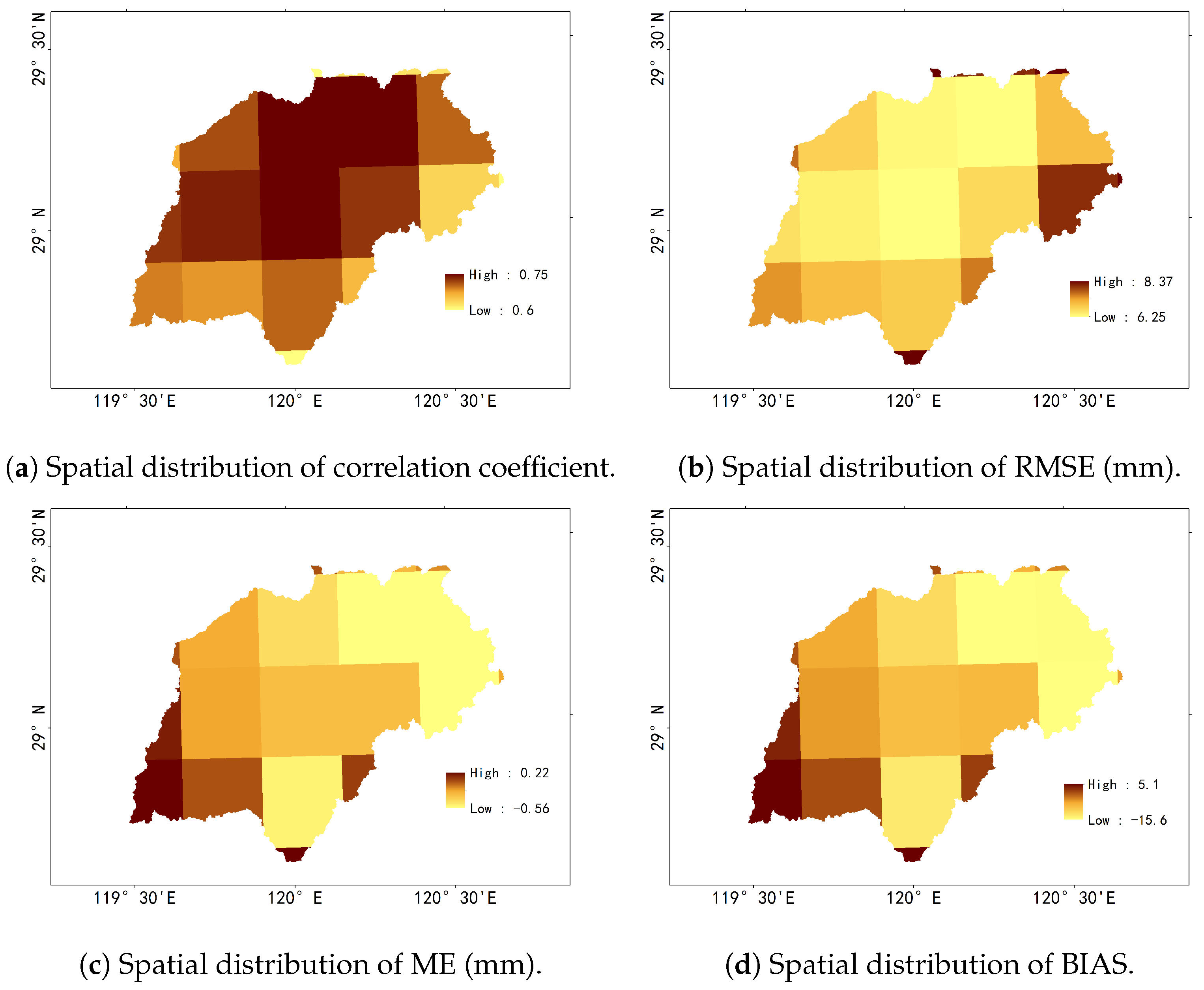
The spatial variabilities of CC, RMSE, ME, and BIAS of daily precipitation within Jinhua River basin are show in Figure 2. The result shows that CMADS estimates daily precipitation better in plain areas than in mountainous areas. The correlation coefficient ranges from 0.60 to 0.75, with larger values in middle plain areas and smaller values in marginal mountainous areas. The spatial distributions of ME and BIAS show that CMADS tend to underestimate precipitation in middle plain areas and marginal mountainous areas.

CMADS estimates temperature and relative humidity more accurately than precipitation and wind speeds. This may attribute to that: (1) Temperature and relative humidity are highly correlated and more stable than precipitation and wind [44]; (2) The studied basin is mountainous dominated, where the spatiotemporal distribution of precipitation and wind speed is more uneven than in plain areas and hard to be simulated by NWP models [21].

3.1.2. Comparison at Monthly Scale

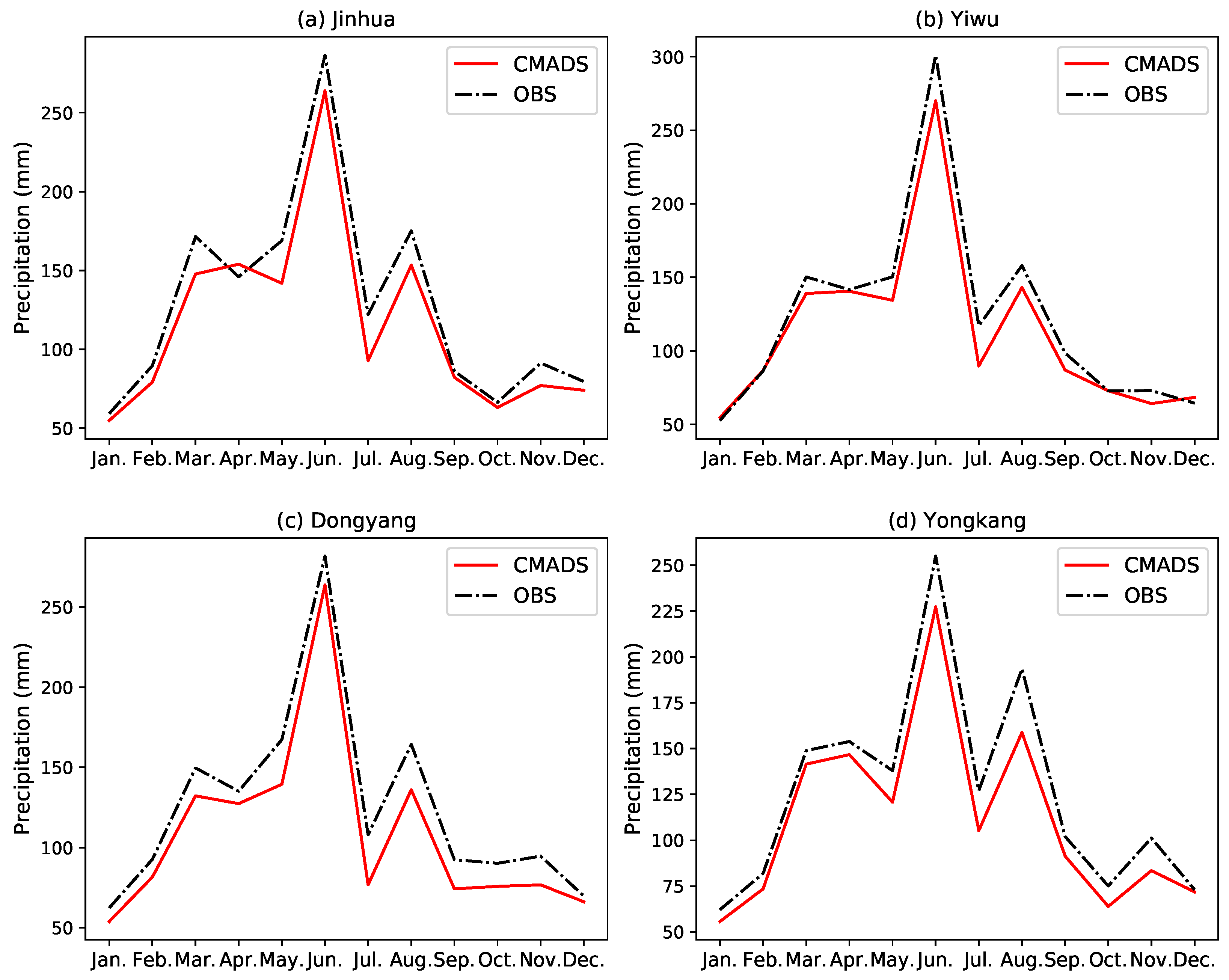
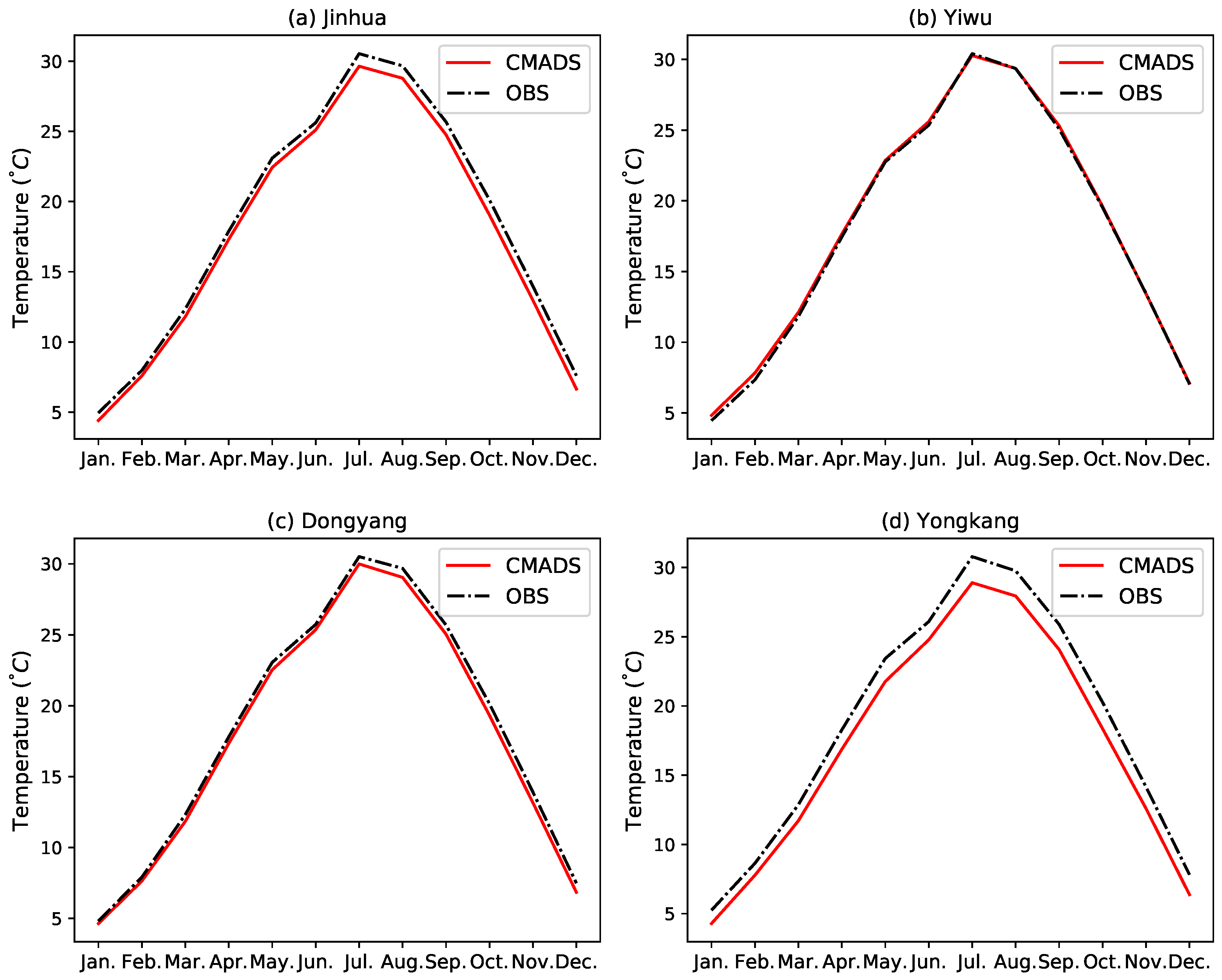
Precipitation and Temperature are the most important meteorological factors for hydrological simulations. The comparisons of temporal distribution patterns of multi-year average monthly precipitation, temperature are shown in Figure 3 and Figure 4. The results show that CMADS can capture temporal distribution patterns well for precipitation and temperature. Overall, CMADS almost underestimates these evaluated meteorological elements more or less for all months in the evaluated gauges. The exception is that the temperature estimates of Yiwu station are consistent very well with gauge observations for every month in a year.

Values of diagnostic statistics (CC, RMSE, ME, and BIAS, BIAS is not calculated for wind speed) between monthly CMADS estimates and gauge observations for the four stations and the basin average are summarized in

Table 3. Statistical indexes of monthly estimates.

Monthly Precipitation
Gauges	CC	RMSE (mm)	ME (mm)	BIAS (%)
Jinhua	0.94	32.78	−13.18	−11.42
Yiwu	0.95	29.21	−9.65	−8.57
Dongyang	0.97	26.54	−17.01	−15.65
Yongkang	0.94	29.20	−14.31	−12.81
Basin average	0.96	22.62	−7.90	−6.67
Monthly Temperature
Gauges	CC	RMSE (°C)	ME (°C)	BIAS (%)
Jinhua	1.00	0.80	−0.75	−4.26
Yiwu	1.00	0.29	0.16	0.88
Dongyang	1.00	0.59	−0.52	−2.96
Yongkang	1.00	1.54	−1.48	−8.66
Basin average	1.00	1.10	−0.55	−5.15
Monthly Wind Speed
Gauges	CC	RMSE (m/s)	ME (m/s)
Jinhua	0.71	1.32	−1.31
Yiwu	0.62	1.83	−1.82
Dongyang	0.28	1.01	−0.97
Yongkang	0.59	0.88	−0.87
Basin average	0.55	1.17	−1.16
Monthly Relative Humidity
Gauges	CC	RMSE	ME	BIAS (%)
Jinhua	0.92	5.12	4.61	6.50
Yiwu	0.94	2.92	2.10	2.97
Dongyang	0.90	5.82	5.14	7.10
Yongkang	0.92	7.50	7.15	9.85
Basin average	0.93	7.35	7.05	9.60

. CMADS reproduces monthly precipitation, temperature and relative humidity well compared with gauge observations. Its estimates of monthly precipitation, temperature, and relative humidity have perfect linear correlation with gauge observations (with CC > 0.90). The BIAS of monthly temperature and relative humidity between CMADS estimates and gauge observations is <10% for all the stations and the basin average, while the BIAS of monthly precipitation ranges from 5% to 15%. The absolutely deviation of wind speeds for the four gauges is within 2.0 m/s.

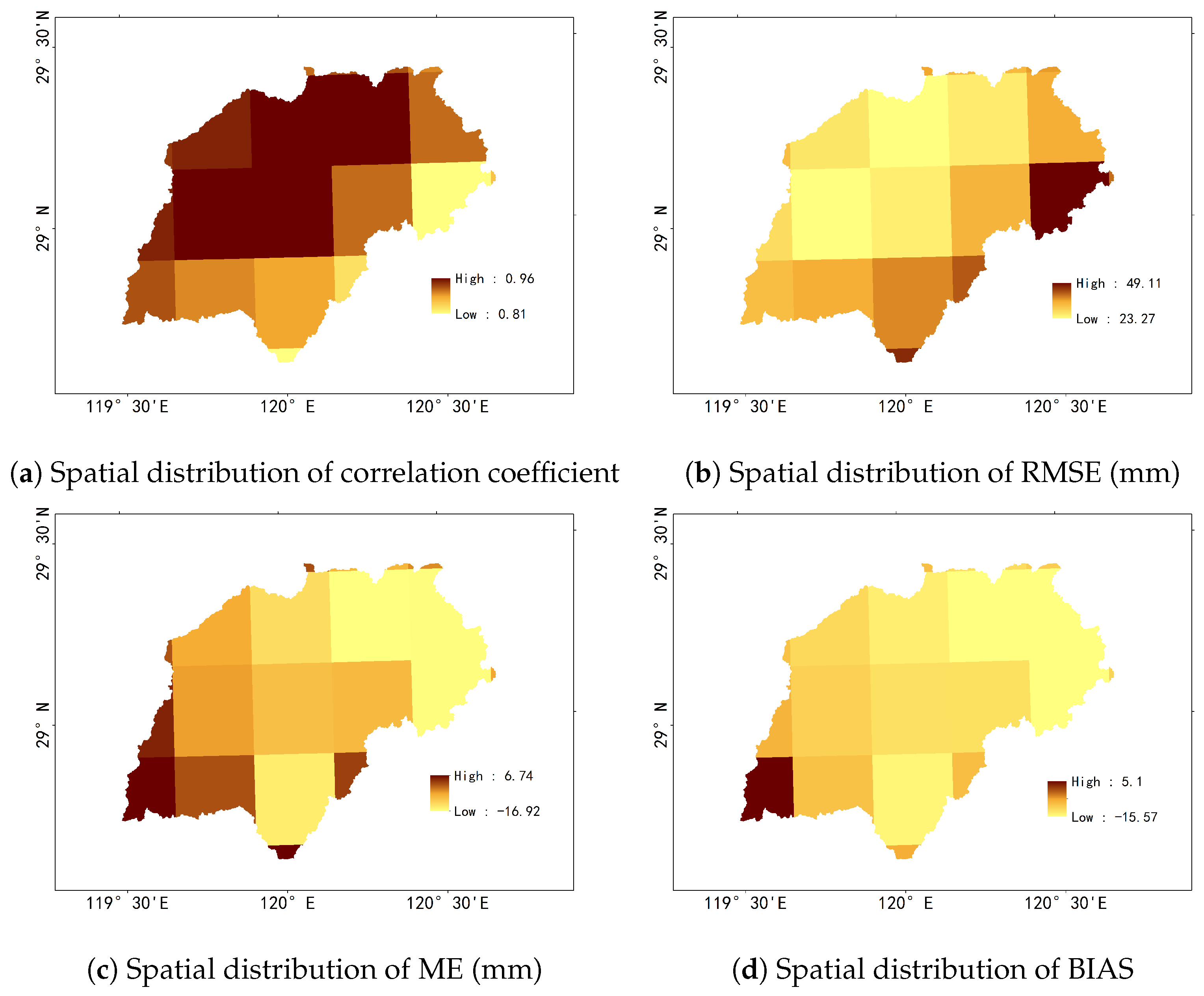
The spatial variabilities of CC, RMSE, ME, and BIAS of monthly precipitation within Jinhua River basin are similar with that of daily precipitation (Figure 5). The result shows that CMADS estimates monthly precipitation better in plain areas than in mountainous areas. The correlation coefficient ranges from 0.81 to 0.96, with larger values in middle plain areas and smaller values in marginal mountainous areas. The spatial distributions of ME and BIAS of monthly precipitation show that CMADS tend to underestimate precipitation in most parts of the basin except some marginal mountainous areas.

3.2. Results of Model Calibration and Validation

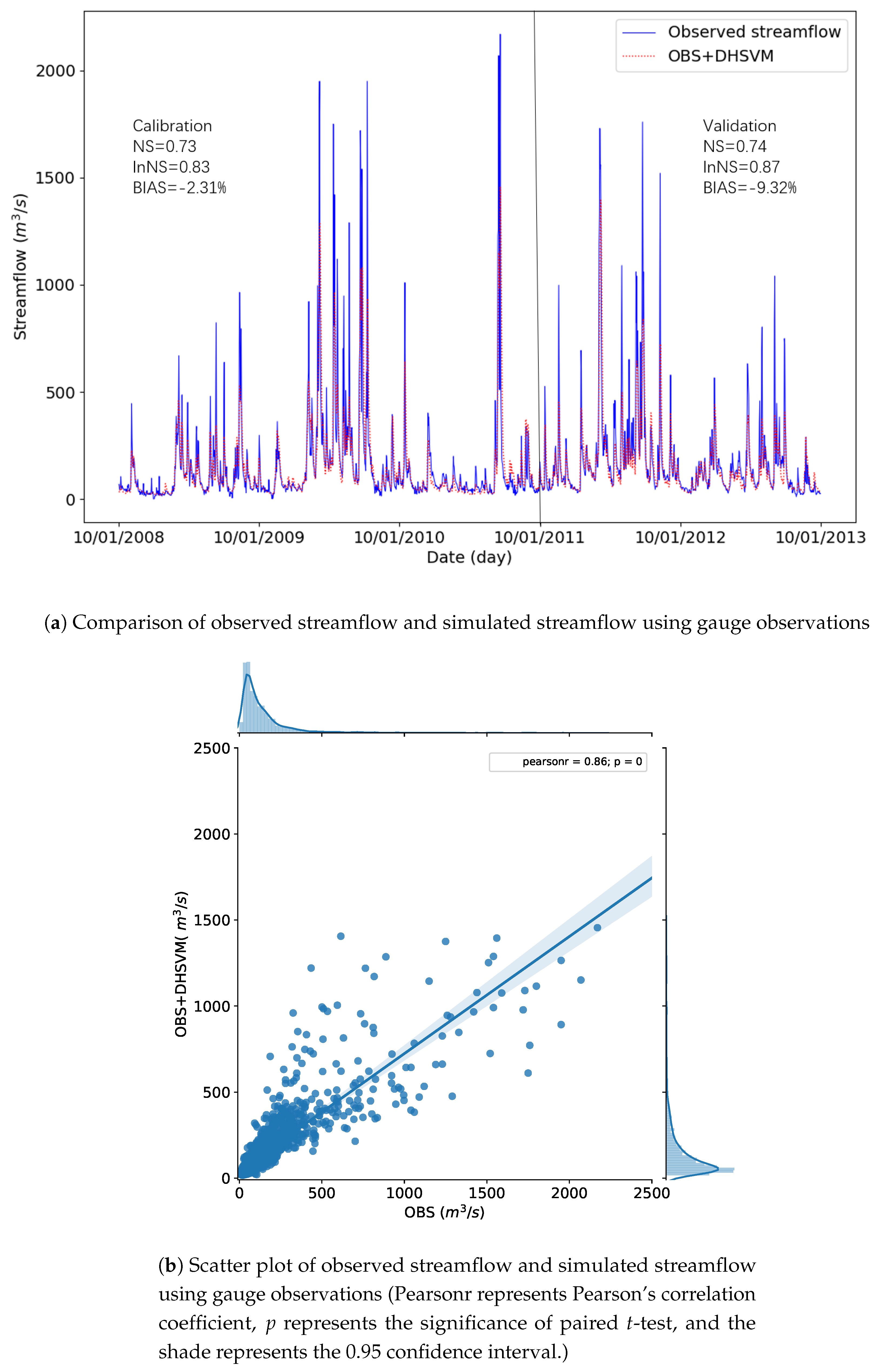
The performance of DHSVM for streamflow simulation using gauge meteorological data as inputs in Jinhua River basin during calibration and validation has been shown in

Table 4. Performance indexes of DHSVM using gauge observations as inputs.

Period	NS	lnNS	BIAS (%)
Calibration	0.73	0.83	−2.31
Validation	0.74	0.87	−9.32

. The NS efficiency coefficients are 0.73 and 0.74 during calibration and validation period, respectively, indicating that the model can capture the streamflow characteristics well. The model performs well in low flow simulation, with 0.83 and 0.87 for lnNS during calibration and validation period, respectively. The BIASs are <5% for calibration period ($-2.31$%) and <10% for validation period ($-9.32$%), which means that the model performs well in streamflow volume simulation.

The indexes for dry seasons (from April to September) and wet seasons (other months) were shown in

Table 5. Performance indexes of DHSVM using gauge observations as inputs during dry and wet seasons.

Dry Seasons
Period	NS	lnNS	BIAS (%)
Calibration	0.81	0.82	−3.30
Validation	0.80	0.88	−4.11
Wet seasons
Period	NS	lnNS	BIAS (%)
Calibration	0.70	0.84	−1.82
Validation	0.69	0.86	−12.98

. The results show that the model performs well in both dry and wet seasons, but the performance in dry seasons is better than that in wet seasons. The NS efficiency coefficients are 0.81/0.70 and 0.80 (0.69) during calibration and validation period, respectively, in dry(wet) seasons, while the BIAS are $-3.30$% ($-1.82$%) and $-4.11$% ($-12.98$%) during calibration and validation period, respectively.

Figure 6 shows the calibration and validation results. It can be observed from the figure that the model simulates the daily runoff well. The simulated streamflow has a good linear relationship with simulated streamflow with 0.86 for Pearson’s efficiency coefficient. However, the peak flows are often underestimated, indicating that the model may be relatively weak in simulating flood peaks. The underestimation of peak flows may be due to (1) The precipitation stations in this area do not cover the whole basin and thus cannot reproduce the real precipitation process in the basin, (2) the trial and error method was used to calibrate the model considering the computational efficiency and this method may not capture the optimal parameters, and (3) the model structure has some problems in simulating peak flows, for example, it cannot consider preferential flow which is an important component of peak flows [45].

3.3. Comparison of Streamflow Simulations

Runoff is a response of complicated dynamical and thermodynamical interactions of meteorological and underlying elements. Physically-based distributed hydrological model such as DHSVM is one of the most effective instruments of exploring the detailed processes of water cycle. However, the accuracy of model results depend on the accuracy of meteorological data that are used as inputs of the hydrological model. Both the spatiotemporal distributions and the magnitudes of meteorological data have a significant impact on the output of a distributed hydrological model. This section evaluated the performance of CMADS dataset as driver of a hydrological model by comparing the simulated streamflow forced by CMADS with observed streamflow and simulated streamflow forced by gauge observations of meteorological data.

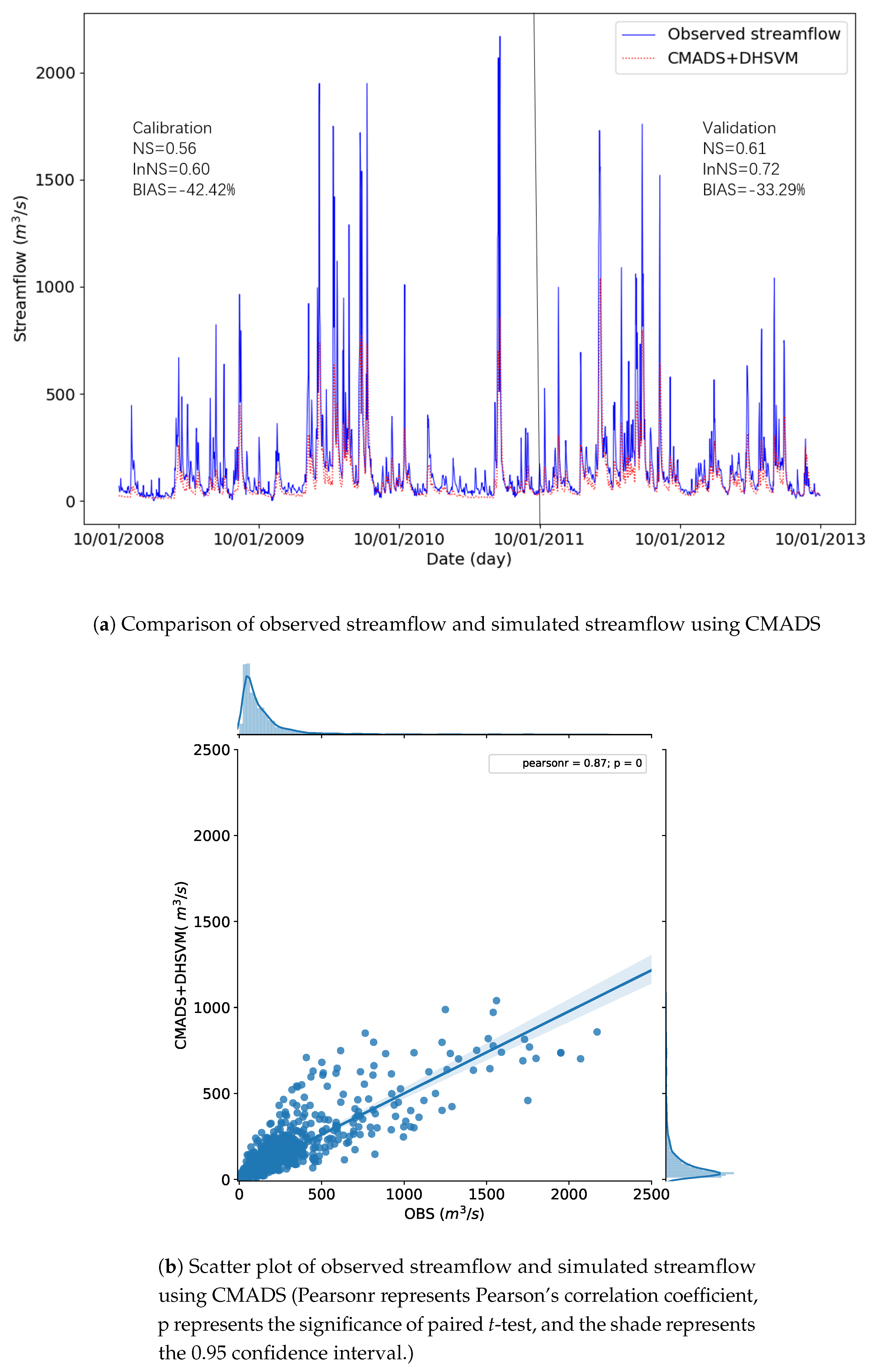
The hydrological application performance of CMADS is shown in

Table 6. Performance indexes of DHSVM using CMADS as inputs.

Period	NS	lnNS	BIAS (%)
Calibration	0.56	0.60	−42.42
Validation	0.61	0.72	−33.29

. Overall, the model using meteorological data derived from CMADS can capture the streamflow characteristics acceptably, with the NS of 0.56 and 0.61 for calibration period and validation period, respectively. However, the model underestimates streamflow significantly, with the BIAS of $-42.42$% for calibration period and $-33.29$% for validation period. It can be seen from

Table 7. Performance indexes of DHSVM using CMADS dataset as inputs during dry and wet seasons.

Dry Seasons
Period	NS	lnNS	BIAS (%)
Calibration	0.53	0.55	−48.40
Validation	0.67	0.66	−32.72
Wet Seasons
Period	NS	lnNS	BIAS (%)
Calibration	0.56	0.61	−39.41
Validation	0.57	0.76	−33.68

that the underestimation of low flows (during dry seasons) is more serious than high flows (during wet seasons) during calibration period. The underestimation of low flows and high flows are similar during validation period.

Figure 7 shows the comparison between observed streamflow and simulated streamflow using CMADS meteorological data. The result shows that the model driven by CMADS meteorological data can capture the streamflow characteristics acceptably but underestimate it obviously.

Flow duration curve is of significant importance in flood controlling and water resources management. Figure 8 compares the flow duration curves of observed, simulated with gauge observations, and simulated with CMADS data runoff. The result show that the majority of daily flows (>90%) are less than 500 m${}^3$/s. The flow duration curves of observed runoff and simulated runoff with gauge observations have a similar probability distribution pattern while the simulated flow with CMADS underestimates runoff at almost all quantiles.

3.4. Comparison of Evapotranspiration

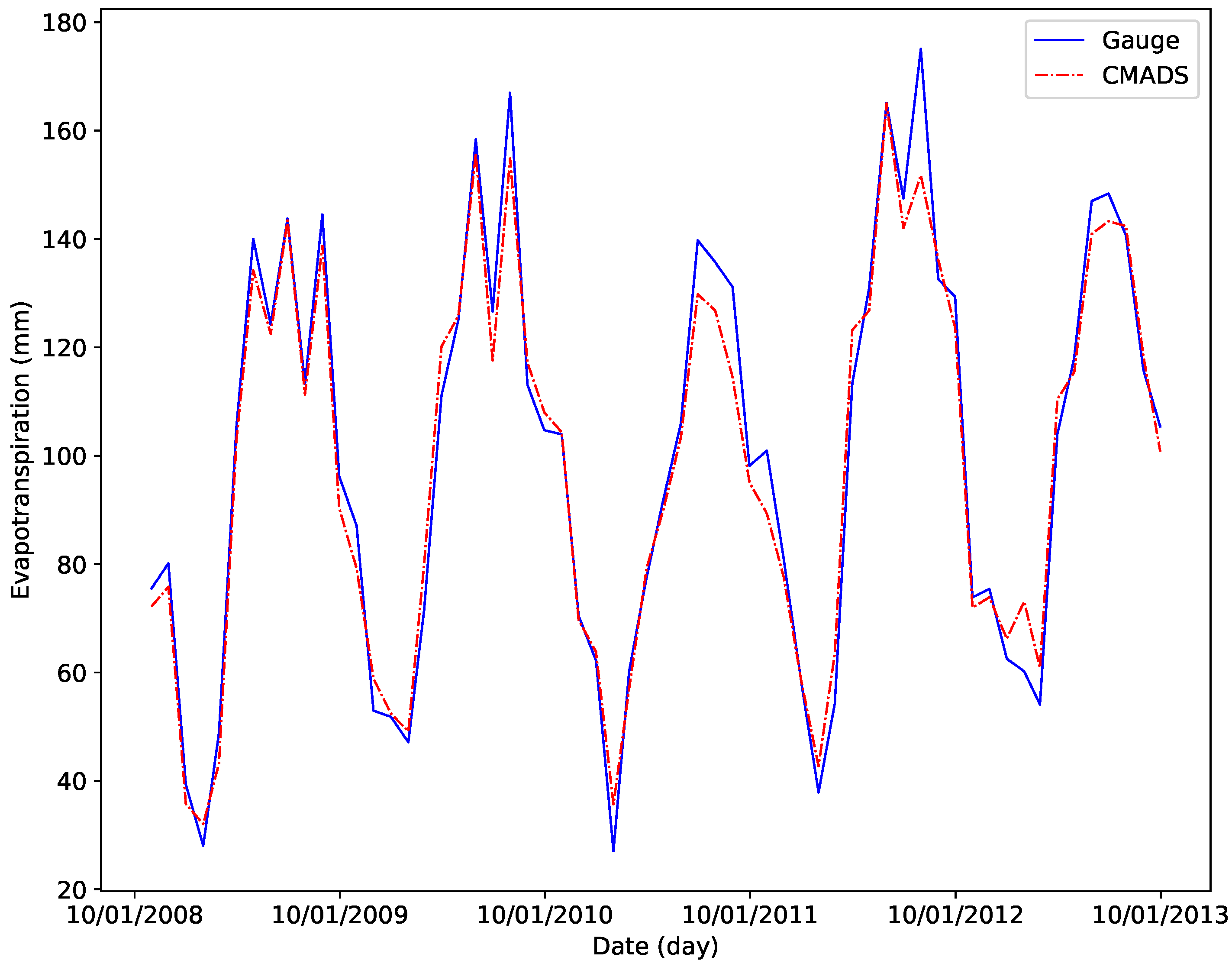
Evapotranspiration is a primary component of the water cycle, providing a critical nexus between terrestrial water, carbon and surface energy exchanges [46]. The simulated mean monthly evapotranspiration of the basin driven by gauge observations and CMADS dataset were compared (Figure 9).

Table 8. Performance indexes of simulated evapotranspiration.

Period	NS	lnNS	BIAS (%)
Calibration	0.97	0.97	−2.01
Validation	0.96	0.96	−0.54

shows that the mean monthly evapotranspiration simulated by DHSVM forced by CMADS data is highly consistent with that forced by gauge observations, with NS efficiency coefficients of 0.97 during calibration period and 0.96 during validation period. The simulated evapotranspitration forced by CMADS dataset is slightly smaller than that forced by gauge observations. The biases between simulated evapotranspiration forced by CMADS dataset and forced by gauge observations are −2.01% during calibration period and −0.54% during validation period.

3.5. Comparison of Soil Moisture Content

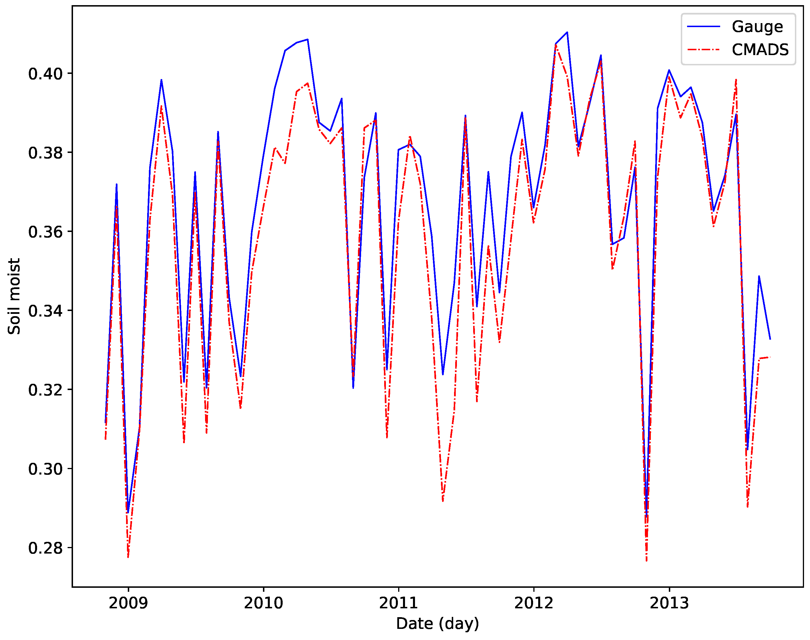
Soil moisture content can reflect the wet state of the basin and gives clues of the rainfall-runoff mechanism to some extent. We compared the varieties of the mean monthly soil moisture content of the basin simulated by DHSVM with gauge observations and CMADS data in Figure 10. The results show that the mean monthly soil moisture content simulated by DHSVM forced by CMADS data is highly consistent with that forced by gauge observations, with NS efficiency coefficients of 0.81 during calibration period and 0.91 during validation period (

Table 9. Performance indexes of simulated soil moisture content.

Period	NS	lnNS	BIAS (%)
Calibration	0.81	0.80	−2.85
Validation	0.91	0.91	−1.39

). The simulated monthly mean soil moisture content forced by CMADS dataset is slightly smaller than that forced by gauge observations. The biases between simulated soil moisture content forced by CMADS dataset and forced by gauge observations are −2.85% during calibration period and −1.39% during validation period.

4. Discussion

Evaluation and application of reanalysises have been performed in many studies because of their application prospects in ungauged regions [47,48]. There are mainly two ways to evaluate reanalysis datasets: straightforward comparison between reanalysis datasets and gauge observations and comparison between simulated hydrological fluxes driven by reanalysis datasets and their observed counterparts [49,50,51]. The straightforward comparison mainly includes three strategies: comparison between grid-gauge pairs [18,52], comparison between grid-grid pairs (gauge observations are interpolated into same grids as reanalysis datasets), and comparison between basin averages [36,53]. Each strategies mentioned above has its drawbacks. For example, grid-gauge pairs comparison may introduce errors because that grid values of reanalysis datasets are actually grid-average values while gauge values are point-values of some locations within the grids. Errors would be introduced as a consequence of interpolation, if grid-grid comparison strategy is used. Comparison between basin averages cannot illustrate spatial variability of the performance of reanalysis datasets.

The Evaluation of CMADS and its hydrological application have been performed in many regions across East Asia. The dataset performs well in terms of correlation with gauge observations while the bias between CMADS and gauge observations varies obviously [26,36]. Many comparison studies between CMADS and other reanalysis datasets show that CMADS has obvious advantages in hydrological application in China than other reanalysis datasets [26,54]. In this study, the model forced by CMADS dataset underestimates streamflow obviously, especially in dry seasons. Calibration strategies may contribute to the underestimation. Streamflow simulations are highly impacted by calibration strategies. There are two calibration strategies usually used in evaluating hydrological application of reanalysis and/or satellite-based datasets: (1) the model is calibrated separately for CMADS and gauge observations, and (2) the calibration is carried out using simulated streamflow driven by gauge meteorological data and observed streamflow, and then, the calibrated parameters are used to hydrological model with CMADS [53]. Theoretically, the first calibration strategy tends to get better evaluation results, because the simulated streamflow are fitting to observed streamflow separately. However, the model may sacrifice the simulation accuracy of other fluxes (such as evapotranspitration) and state variables (such as soil moisture content) because of placing too much value on streamflow simulation, when the first calibration strategy is used. In this study, the second calibration strategy was used to calibrate the model. In this way, the hydrological response mechanism was assumed to be constant across different inputs. Hence, low precipitation inputs are guaranteed to lead to underestimation of streamflow.

The underestimation of streamflow can be explained from the perspective of mass balance. In a natural basin, runoff is generated by precipitation reducing evapotranspiration and the change of water storage in a basin. Section 2.5 has show that CMADS tends to underestimate precipitation by more than 10 percent, but the simulated evapotranspiration and soil moisture content forced by CMADS dataset are highly consistent with that forced by gauge observations, which means that water loss in the hydrological cycle is similar. Therefore, the underestimation of precipitation would lead to the underestimation of the streamflow.

Another result of this study is that the model forced by CMADS underestimates streamflow more seriously in dry seasons than in wet seasons. To identify the reason for this phenomenon, precipitation was divided into dry and wet reasons and biases were calculated separately. CMADS underestimates precipitation by −17.40% during dry seasons but −10.96% during wet seasons. Under the condition that the evapotranspiration and soil moisture content simulated by DHSVM forced by CMADS are similar with that forced by gauge observations, the model underestimates streamflow more seriously because that CMADS underestimates precipitation more seriously.

Actual evapotranspiration is one of the most important components of water circulation. It links energy exchange and mass (such as water and carbon) transport. In this paper, the evaluation of CMADS in simulating evapotranspiration is performed using compared simulated evapotranspiration forced by CMADS with that forced by gauge observations. The deviation between simulated evapotranspiration forced by CMADS and actual evapotranspiration needs to be further investigated.

5. Conclusions

The performance of CMADS and its hydrological application were evaluated in this paper. The results show that CMADS can represent meteorological elements including precipitation, temperature, relative humidity, and wind speed reasonably for both daily and monthly temporal scales. The correlations of temperature and relative humidity between CMADS estimates and gauge observations are >0.90, and the BIAS of that between CMADS estimates and gauge observations are <10% for both daily and monthly temporal scale. The precipitation estimates have a good linear correlation with gauged precipitation (>0.70 for daily temporal scale and >0.90 for monthly temporal scale) but underestimate precipitation compared with gauge observations slightly (with BIAS within −15% for both daily and monthly temporal scales). The correlation coefficients of wind speeds are acceptable for most stations (>0.55) except Jinhua station (<0.50) and the absolutely deviation of wind speeds is around −1.0 m/s for the two temporal scales.

The hydrological model using CMADS dataset as meteorological inputs can capture the daily streamflow characteristics well overall (with a NS value of 0.56 during calibration period and 0.61 during validation period) but underestimates streamflow obviously (with a BIAS of −42.42% during calibration period and a BIAS of −33.29% during validation period). The underestimation of streamflow simulated by the model driven by CMADS dataset is more seriously in dry seasons (−48.40%) than that in wet seasons (−39.41%) for calibration period. The model driven by CMADS predicts evapotranspiration and soil moisture content well compared with the model driven by gauge observations.

References

- Baldassarre, G.D.; Montanari, A.; Lins, H.; Koutsoyiannis, D.; Brandimarte, L.; Blöschl, G. Flood fatalities in Africa: From diagnosis to mitigation. Geophys. Res. Lett. 2010, 37, 707–716. [Google Scholar] [CrossRef]
- Winsemius, H.C.; Aerts, J.C.J.H.; Beek, L.P.H.V.; Bierkens, M.F.P.; Bouwman, A.; Jongman, B.; Kwadijk, J.C.J.; Ligtvoet, W.; Lucas, P.L.; Vuuren, D.P.V. Global drivers of future river flood risk. Nat. Clim. Chang. 2016, 6, 381. [Google Scholar] [CrossRef]
- Ma, F.; Ye, A.; You, J.; Duan, Q. 2015–16 floods and droughts in China, and its response to the strong El Niño. Sc. Total Environ. 2018, 627, 1473–1484. [Google Scholar] [CrossRef]
- Kite, G. Modelling the Mekong: Hydrological simulation for environmental impact studies. J. Hydrol. 2001, 253, 1–13. [Google Scholar] [CrossRef]
- Bellos, V.; Tsakiris, G. A hybrid method for flood simulation in small catchments combining hydrodynamic and hydrological techniques. J. Hydrol. 2016, 540, 331–339. [Google Scholar] [CrossRef]
- Schumacher, M.; Forootan, E.; Dijk, A.I.J.M.V.; Schmied, H.M.; Crosbie, R.S.; Kusche, J.; Döll, P. Improving drought simulations within the Murray-Darling Basin by combined calibration/assimilation of GRACE data into the WaterGAP Global Hydrology Model. Remote Sens. Environ. 2017, 204, 212–228. [Google Scholar] [CrossRef]
- Wigmosta, M.S.; Nijssen, B.; Storck, P.; Singh, V.P.; Frevert, D. The distributed hydrology soil vegetation model. Hydrol. Process. 2002, 22, 4205–4213. [Google Scholar]
- Arnold, J.G.; Moriasi, D.N.; Gassman, P.W.; Abbaspour, K.C.; White, M.J.; Srinivasan, R.; Santhi, C.; Harmel, R.D.; Griensven, A.V.; Liew, M.W.V. SWAT: Model use, calibration, and validation. Trans. ASABE 2012, 55, 1345–1352. [Google Scholar] [CrossRef]
- Wigmosta, M.S.; Vail, L.W.; Lettenmaier, D.P. A distributed hydrology-vegetation model for complex terrain. Water Resour. Res. 1994, 30, 1665–1679. [Google Scholar] [CrossRef]
- Abbott, M.B.; Refsgaard, J.C. Distributed Hydrological Modelling; Springer: Berlin/Heidelberg, Germany, 1996; pp. 289–305. [Google Scholar]
- Zhang, W.C.; Ogawa, K.; Ye, B.S.; Yamaguchi, Y. A monthly stream flow model for estimating the potential changes of river runoff on the projected global warming. Hydrol. Process. 2015, 14, 1851–1868. [Google Scholar]
- Chen, J.M.; Chen, X.; Ju, W.; Geng, X. Distributed hydrological model for mapping evapotranspiration using remote sensing inputs. J. Hydrol. 2005, 305, 15–39. [Google Scholar] [CrossRef]
- Wang, A.; Zeng, X. Evaluation of multireanalysis products with in situ observations over the Tibetan Plateau. J. Geophys. Res. Atmos. 2012, 117, D0512. [Google Scholar] [CrossRef]
- Janowiak, J.E.; Gruber, A.; Kondragunta, C.R.; Livezey, R.E.; Huffman, G.J. A Comparison of the NCEP-NCAR Reanalysis Precipitation and the GPCP Rain Gauge-Satellite Combined Dataset with Observational Error Considerations. J. Clim. 1998, 11, 2960–2979. [Google Scholar] [CrossRef]
- Sheffield, J.; Goteti, G.; Wood, E.F. Development of a 50-Year High-Resolution Global Dataset of Meteorological Forcings for Land Surface Modeling. J. Clim. 2005, 19, 3088–3111. [Google Scholar] [CrossRef]
- Tang, M.S.Y.; Chenoli, S.N.; Samah, A.A.; Hai, O.S. An assessment of historical Antarctic precipitation and temperature trend using CMIP5 models and reanalysis datasets. Polar Sci. 2018, 15, 1–12. [Google Scholar] [CrossRef]
- Maurer, E.P.; Lettenmaier, D.P. Predictability of seasonal runoff in the Mississippi River basin. J. Geophys. Res. Atmos. 2003, 108, D16. [Google Scholar] [CrossRef]
- Li, C.; Tang, G.; Hong, Y. Cross-Evaluation of Ground-based, Multi-Satellite and Reanalysis Precipitation Products: Applicability of the Triple Collocation Method across Mainland China. J. Hydrol. 2018, 562, 71–83. [Google Scholar] [CrossRef]
- Smith, S.R. Quantifying uncertainties in NCEP reanalyses using high-quality research vesses observations. J. Clim. 2001, 14, 4062–4072. [Google Scholar] [CrossRef]
- Hodges, K.I.; Lee, R.W.; Bengtsson, L. A Comparison of Extratropical Cyclones in Recent Reanalyses ERA-Interim, NASA MERRA, NCEP CFSR, and JRA-25. J. Clim. 2011, 24, 4888–4906. [Google Scholar] [CrossRef]
- Ebisuzaki, W.; Zhang, L. Assessing the performance of the CFSR by an ensemble of analyses. Clim. Dyn. 2011, 37, 2541–2550. [Google Scholar] [CrossRef]
- Dee, D.; Uppala, S.; Simmons, A.J.; Berrisford, P.; Poli, P.; Kobayashi, S.; Andrae, U.; Balmaseda, M.A.; Balsamo, G.; Bauer, P.; et al. The ERA-Interim reanalysis: Configuration and performance of the data assimilation system. Q. J. R. Meteorol. Soc. 2011, 137, 553–597. [Google Scholar] [CrossRef]
- Smith, C.A.; Compo, G.P.; Hooper, D.K. Web-Based Reanalysis Intercomparison Tools (WRIT) for analysis and comparison of reanalyses and other datasets. Bull. Am. Meteorol. Soc. 2014, 95, 1671–1678. [Google Scholar] [CrossRef]
- Meng, X.; Wang, H.; Meng, X.; Wang, H. Significance of the China Meteorological Assimilation Driving Datasets for the SWAT Model (CMADS) of East Asia. Water 2017, 9, 765. [Google Scholar] [CrossRef]
- Zhao, F.; Wu, Y.; Qiu, L.; Sun, Y.; Sun, L.; Li, Q.; Niu, J.; Wang, G. Parameter Uncertainty Analysis of the SWAT Model in a Mountain-Loess Transitional Watershed on the Chinese Loess Plateau. Water 2018, 10, 690. [Google Scholar] [CrossRef]
- Thom, V.; Li, L.; Jun, K.S. Evaluation of Multi-Satellite Precipitation Products for Streamflow Simulations: A Case Study for the Han River Basin in the Korean Peninsula, East Asia. Water 2018, 10, 642. [Google Scholar]
- Meng, X.; Long, A.; Wu, Y.; Yin, G.; Wang, H.; Ji, X. Simulation and spatiotemporal pattern of air temperature and precipitation in Eastern Central Asia using RegCM. Sci. Rep. 2018, 8, 3639. [Google Scholar] [CrossRef] [PubMed] [Green Version]
- Meng, X.Y.; Yu, D.L.; Liu, Z.H. Energy balance-based SWAT model to simulate the mountain snowmelt and runoff—Taking the application in Juntanghu watershed (China) as an example. J. Mt. Sci. 2015, 12, 368–381. [Google Scholar] [CrossRef]
- Meng, X.; Sun, Z.; Zhao, H.; Ji, X.; Wang, H.; Xue, L.; Wu, H.; Zhu, Y. Spring Flood Forecasting Based on the WRF-TSRM Mode. Tehnički Vjesnik 2018, 25, 27–37. [Google Scholar]
- Meng, X.; Wang, H.; Lei, X.; Cai, S.; Wu, H.; Ji, X.; Wang, J. Hydrological modeling in the manas river basin using soil and water assessment tool driven by CMADS. Tehnički Vjesnik 2017, 24, 525–534. [Google Scholar]
- Meng, X.; Wang, H.; Wu, Y.; Long, A.; Wang, J.; Shi, C.; Ji, X. Investigating spatiotemporal changes of the land-surface processes in Xinjiang using high-resolution CLM3.5 and CLDAS: Soil temperature. Sci. Rep. 2017, 7, 13286. [Google Scholar] [CrossRef] [Green Version]
- Liu, J.; Shanguan, D.; Liu, S.; Ding, Y. Evaluation and Hydrological Simulation of CMADS and CFSR Reanalysis Datasets in the Qinghai-Tibet Plateau. Water 2018, 10, 513. [Google Scholar] [CrossRef]
- Wang, Y.J.; Meng, X.Y.; Liu, Z.H.; Ji, X.N. Snowmelt Runoff Analysis under Generated Climate Change Scenarios for the Juntanghu River Basin, in Xinjiang, China. Water Sci. Technol. 2016, 7, 41–54. [Google Scholar]
- Xu, Y.P.; Gao, X.; Zhu, Q.; Zhang, Y.; Kang, L. Coupling a Regional Climate Model and a Distributed Hydrological Model to Assess Future Water Resources in Jinhua River Basin, East China. J. Hydrol. Eng. 2015, 20, 04014054. [Google Scholar] [CrossRef]
- Chen, H.; Xu, C.Y.; Guo, S. Comparison and evaluation of multiple GCMs, statistical downscaling and hydrological models in the study of climate change impacts on runoff. J. Hydrol. 2012, 434, 36–45. [Google Scholar] [CrossRef]
- Gao, X.; Zhu, Q.; Yang, Z.; Wang, H. Evaluation and Hydrological Application of CMADS against TRMM 3B42V7, PERSIANN-CDR, NCEP-CFSR, and Gauge-Based Datasets in Xiang River Basin of China. Water 2018, 10, 1225. [Google Scholar] [CrossRef]
- Caracciolo, D.; Francipane, A.; Viola, F.; Noto, L.V.; Deidda, R. Performances of GPM satellite precipitation over the two major Mediterranean islands. Atmos. Res. 2018, 213, 309–322. [Google Scholar] [CrossRef]
- Ebert, E.E.; Janowiak, J.E.; Kidd, C. Comparison of Near-Real-Time Precipitation Estimates from Satellite Observations and Numerical Models. Bull. Am. Meteorol. Soc. 2010, 88, 47. [Google Scholar] [CrossRef]
- Zhao, Q.; Liu, Z.; Ye, B.; Qin, Y.; Wei, Z.; Fang, S. A snowmelt runoff forecasting model coupling WRF and DHSVM. Hydrol. Earth Syst. Sci. 2009, 13, 233–246. [Google Scholar] [CrossRef]
- Du, E.; Link, T.E.; Gravelle, J.A.; Hubbart, J.A. Validation and sensitivity test of the distributed hydrology soil-vegetation model (DHSVM) in a forested mountain watershed. Hydrol. Process. 2015, 28, 6196–6210. [Google Scholar] [CrossRef]
- Alvarenga, L.A.; Mello, C.R.D.; Colombo, A.; Cuartas, L.A.; Bowling, L.C. Assessment of land cover change on the hydrology of a Brazilian headwater watershed using the Distributed Hydrology-Soil-Vegetation Model. CATENA 2016, 143, 7–17. [Google Scholar] [CrossRef]
- Pan, S.; Fu, G.; Chiang, Y.M.; Ran, Q.; Xu, Y.P. A two-step sensitivity analysis for hydrological signatures in Jinhua River Basin, East China. Hydrol. Sci. J. 2017, 62, 2511–2530. [Google Scholar] [CrossRef]
- Shen, Y.; Xiong, A.; Wang, Y.; Xie, P. Performance of high-resolution satellite precipitation products over China. J. Geophys. Res. Atmos. 2010, 115, D02114. [Google Scholar] [CrossRef]
- Allen, M.R.; Ingram, W.J. Constraints on future changes in climate and the hydrologic cycle. Nature 2002, 419, 224–232. [Google Scholar] [CrossRef]
- Safeeq, M.; Fares, A. Hydrologic response of a Hawaiian watershed to future climate change scenarios. Hydrol. Process. 2012, 26, 2745–2764. [Google Scholar] [CrossRef]
- Zhang, K.; Kimball, J.S.; Running, S.W. A review of remote sensing based actual evapotranspiration estimation. Wiley Interdiscip. Rev. Water 2016, 3, 834–853. [Google Scholar] [CrossRef]
- Krogh, S.A.; Pomeroy, J.W.; McPhee, J. Physically Based Mountain Hydrological Modeling Using Reanalysis Data in Patagonia. J. Hydrometeorol. 2015, 16, 172–193. [Google Scholar] [CrossRef]
- Dile, Y.T.; Srinivasan, R. Evaluation of CFSR climate data for hydrologic prediction in data-scarce watersheds: an application in the Blue Nile River Basin. JAWRA J. Am. Water Resour. Assoc. 2014, 50, 1226–1241. [Google Scholar] [CrossRef]
- Bastola, S.; Misra, V. Evaluation of dynamically downscaled reanalysis precipitation data for hydrological application. Hydrol. Process. 2014, 28, 1989–2002. [Google Scholar] [CrossRef]
- Maurer, E.P.; O’Donnell, G.M.; Lettenmaier, D.P.; Roads, J.O. Evaluation of the land surface water budget in NCEP/NCAR and NCEP/DOE reanalyses using an off-line hydrologic model. J. Geophys. Res. Atmos. 2001, 106, 17841–17862. [Google Scholar] [CrossRef] [Green Version]
- Beck, H.E.; Vergopolan, N.; Pan, M.; Levizzani, V.; van Dijk, A.I.J.M.; Weedon, G.P.; Brocca, L.; Pappenberger, F.; Huffman, G.J.; Wood, E.F. Global-scale evaluation of 22 precipitation datasets using gauge observations and hydrological modeling. Hydrol. Earth Syst. Sci. 2017, 21, 6201–6217. [Google Scholar] [CrossRef] [Green Version]
- Yang, X.; Yong, B.; Hong, Y.; Chen, S.; Zhang, X. Error analysis of multi-satellite precipitation estimates with an independent raingauge observation network over a medium-sized humid basin. Hydrol. Sci. J. 2016, 61, 1813–1830. [Google Scholar] [CrossRef]
- Zhu, Q.; Xuan, W.; Liu, L.; Xu, Y. Evaluation and hydrological application of precipitation estimates derived from PERSIANN-CDR, TRMM 3B42V7, and NCEP-CFSR over humid regions in China. Hydrol. Process. 2016, 30, 3061–3083. [Google Scholar] [CrossRef]
- Guo, B.; Zhang, J.; Xu, T.; Croke, B.; Jakeman, A.; Song, Y.; Yang, Q.; Lei, X.; Liao, W. Applicability Assessment and Uncertainty Analysis of Multi-Precipitation Datasets for the Simulation of Hydrologic Models. Water 2018, 10, 1611. [Google Scholar] [CrossRef]
Figure 1.
Location, elevation, hydrometeorological stations, and CMADS grids in Jinhua River basin.
Figure 2.
Spatial distribution of diagnostic indexes for daily precipitation.
Figure 3.
Multi year average monthly precipitation.
Figure 4.
Multi year average monthly temperature.
Figure 5.
Spatial distribution of diagnostic indexes for monthly precipitation.
Figure 6.
Calibration and validation results.
Figure 7.
Comparison of observed and simulated streamflow.
Figure 8.
Comparison of flow duration curves of observed, simulated with gauge observations, and simulated with CMADS dataset runoff.
Figure 9.
Comparison of mean monthly evapotranspiration.
Figure 10.
Comparison of mean monthly soil moisture content.