Automatic Web Procedure for Calculating Flood Flow Frequency


1
Department of Physics and Geology, Perugia University, 06123 Perugia, Italy
2
CNR—ISMAR (Istituto di Scienze marine/Arsenale), 30122 Venezia, Italy
*
Author to whom correspondence should be addressed.
Water 2019, 11(1), 14; https://doi.org/10.3390/w11010014
Submission received: 13 November 2018
/
Revised: 14 December 2018
/
Accepted: 17 December 2018
/
Published: 21 December 2018
(This article belongs to the Section Hydrology)
Abstract
:The estimated flood flow frequency in a particular cross-section of a riverbed for a given return period is a topic of great interest for its application in hydrological, geomorphological and hydrogeological fields. Nevertheless, to establish a one-to-one relationship between rainfall and peak flow is a difficult problem to solve, due to the great number of factors involved (intensity and distribution of rainfall, hydromorphological characteristics of the watershed, type and distribution of vegetation, soil saturation conditions, etc.). In Italy, the Tiber River Basin Authority has developed a method to evaluate peak flows in the watersheds within the Tiber Basin. The relationship between rainfall depth with an assigned return period (RP) and the duration of the event was determined using data from 165 gauging stations throughout the Basin and in the neighbourhoods with respect to rainfall from 1 to 24 h and/or from 1 to 5 days. To calculate the peak flow with an assigned RP in small watersheds (area < 100 km), the Tiber River Basin Authority proposed a methodology that combines the results of regional precipitation analysis of a duration from 1 to 24 h with the Curve Number method, which allows the volume of net rainfall (i.e., the rainfall that contributes to producing the peak flow) to be quantified. Such procedure includes the calculation of various parameters (run-off time, local rainfall and areal rainfall, net rainfall) in order to obtain the value of peak flow. To facilitate the use of this procedure, a WebGIS system has been developed, based on a series of scripts that calculate the values for the above parameters. The user only has to choose the point corresponding to the section of the channel in order to determine the peak flow and the return period. The computational procedure is performed using GRASS GIS that interfaces with the system using the standard WPS; the system returns to output a report with details of the various calculations of parameters and, as a final result, the value of requested peak flow.
1. Introduction
The determination of peak flow for specific basins is not a trivial problem as it often takes time to collect and evaluate all the data necessary to obtain a reasonable result. Many methods refer to geomorphological models [1,2,3,4,5,6,7,8] and even use Geographic Information Systems (GIS) for calculating peak flow. Many of these models that evaluate peak flow starting from the run-off time, refer above all to non-instrumented water basins [9]. However, several of these methods do not take into account GIS technologies, or are limited to synthetic formulations that lead, moreover, to valid and/or validable results, without taking into account the real geomorphological features.
In literature, several papers, which couple the GIS approach and rainfall-runoff model to estimate the peak flow rate for a specified watershed, are present [10,11,12,13,14]. Cheng et al. [15] proposed a GIS procedure (valid in Oak Ridges Moraine region—Canada) similar to the one here presented, and highlight how a web-gis integration should be developed as an on-line prediction system. Conversely web GIS application are not so common; for example Web GIS application have been successfully used for flood assessment in coastal urban watersheds [16,17]. In Italy there are not knowledge of web applications providing flood frequency estimation.
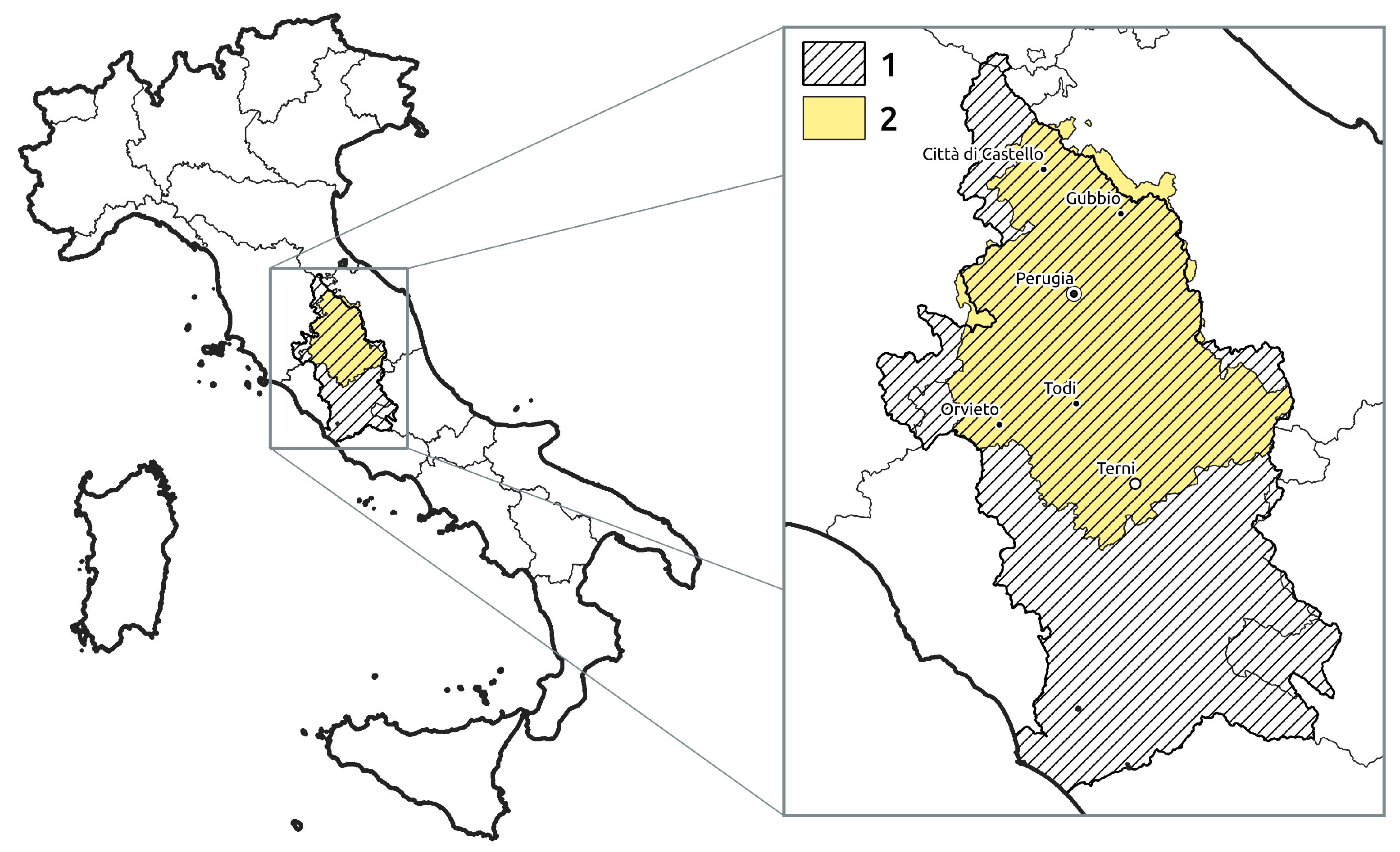
The goal of this paper, and its innovative feature, is to propose an automatic procedure, based on the use of GIS, which allows the peak flow rate to be obtained immediately for a specific cross section for a given return period. The procedure is implemented into a web GIS application and provides a flow rate that, for example, could be useful in design of hydraulic works in non-instrumented watershed. The user has only to select the outlet point on a map and the return period; no other data is required. The method was applied to the Umbrian portion of the Tiber Basin (central Italy—Figure 1, following the Flood Estimation Handbook proposed by the Tiber River Basin Authority [18].
2. Description of Study Area
2.1. Geology
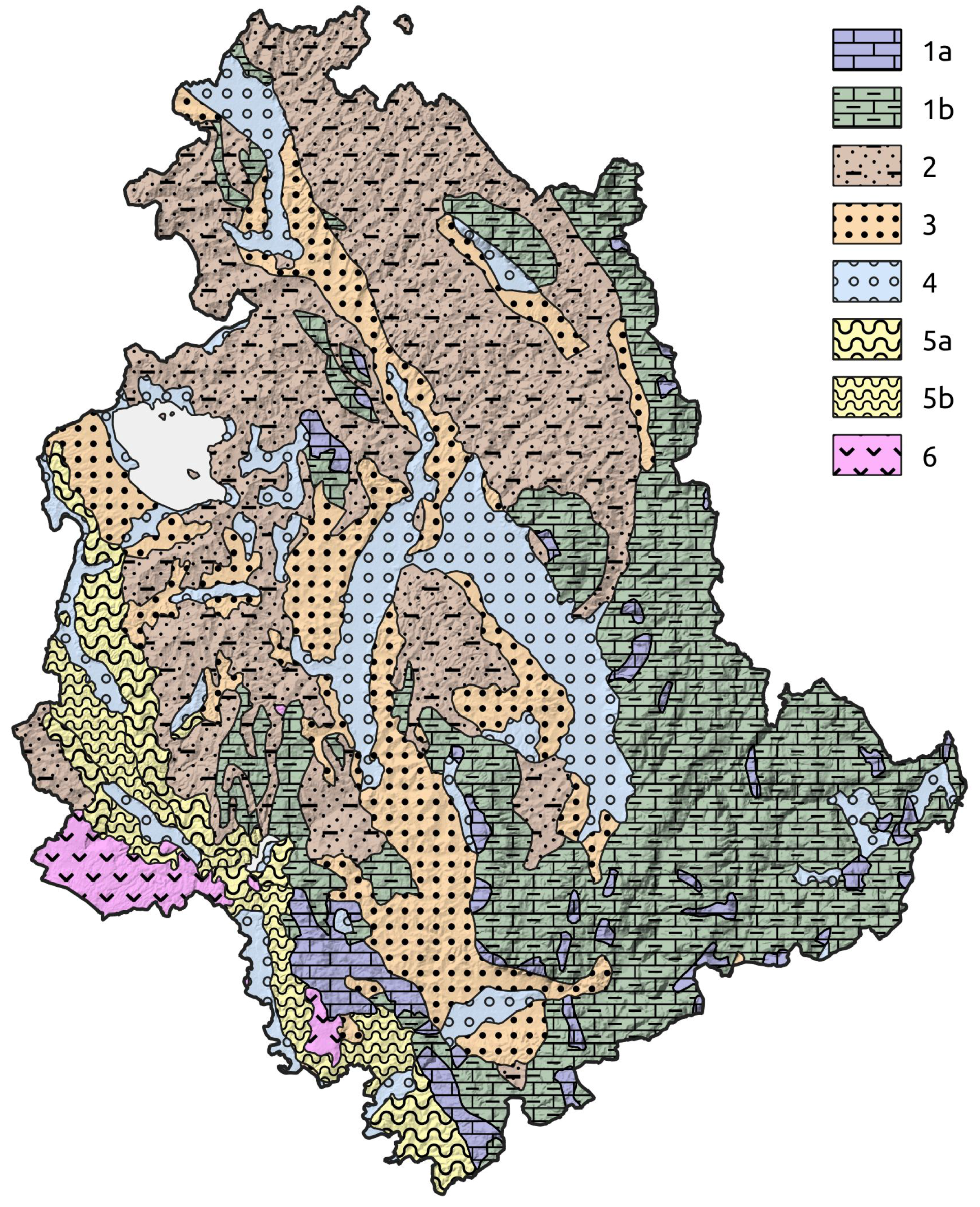
The studied area is the whole Umbria Region. It is characterized by a great geological variability that strongly influences morphological-physiographic characteristics of the territory, vegetation cover, orography and climate. The geological history of the area is strictly connected to the tectonic evolution of the central-northern Apennines. After a period of deposition processes, started in a carbonate platform that evolved in a pelagic environment, a compressive tectonic phase led to the rise of the Apennine fold belt. The following tectonic extensional phase caused the dislocation of the chain into continental fluvio-lacustrine basins (in the central-eastern area) and into coastal marine basins (in the south-western area). Figure 2 shows the geolithological map of Umbria. Rocks and outcropping deposits can be classified according to 6 types of geological formations:
- Carbonate marine formations. They are mainly located in the eastern Apennine area. They can be subdivided into: a sequence of neritic and carbonate platforms facies, consisting mostly of limestones and a minor contribution of marls and dolomites (Late Triassic—Early Jurassic—1a in Figure 2), and a sequence of pelagic facies, consisting of micritic limestones, marly limestones and marls, sometimes with chert (Early Jurassic—Early Miocene—1b Figure 2).
- Siliciclastic marine formations (flysch). They were deposited by density flow processes in foreland basins and, in some cases, in thrust-top-basins. They consist of alternations of sandstones, arenaceous marls and mudrocks, with different ratios that depend on the depositional environment (submarine slope channel, upper fan, lower fan). These formations are dated, moving from west to east, from the Upper Cretaceous to the Upper Miocene.
- Unconsolidated deposits of lacustrine and fluvial-lacustrine continental environment. They were deposited in tectonic sedimentary basins. These are the oldest post-orogenic sediments and consists in gravels and conglomerates, sands, silts and clay. The age of these deposits ranges from the Lower Miocene to the Upper Pleistocene.
- Recent and terraced alluvial deposits. These are the most recent sediments and consist in gravels, sands, silts and clays. The age ranges from the Pleistocene to the Holocene.
- Unconsolidated deposits of marine and brackish-marine environment. They have been deposited at the same time as the continental ones (point 3), in the southwestern part of the studied area, in a coastal marine environment. A coastal/deltaic plain sequence of sands and conglomerates (5a in Figure 2) can be distinguished from a deeper marine environment sequence of clay (5b in Figure 1). The age of these deposits ranges from the Lower Pliocene to the Upper Pleistocene.
- Volcanic rocks. They are located in the most south-western portion of Umbria. They are connected to the activity of the Vulsini volcanic apparatus. They are formed by foidites, tephrites, latites, trachytes and phonolites. The age of these rocks refers to the Middle Pleistocene.
2.2. Soils
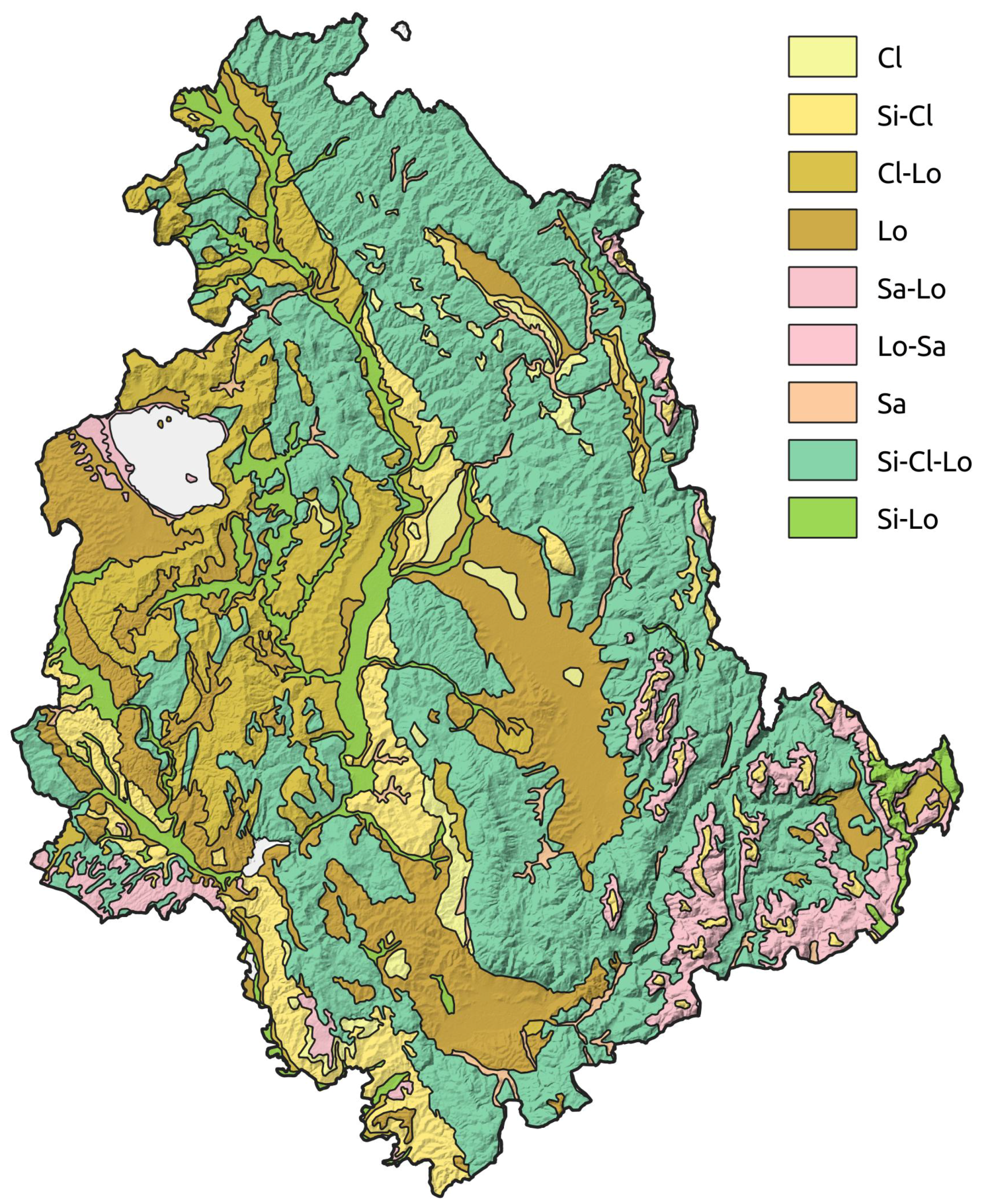
The information regarding the soils was found in the “Soils map of Umbria” (1:200,000 scale) [20]. The map was performed by surveying soil stratigraphic profiles and relating them to the Geological Map of Italy (1:100,000 scale), available at http://portalesgi.isprambiente.it/en/elenco-base-dati/10. The soil type was defined using the ternary diagram of the USDA soil texture classification [21].
Figure 3 shows that in the Umbrian territory the most widespread soils are those in which the silty component predominates (Silty Clay Loam—46.4%). These soils are often associated with both carbonate rocks and turbiditic rocks. Mixed soils (Loam and Clay loam—29.7%) are also frequent, often developing in correspondence to unconsolidated deposits, both in marine facies and in continental (even recent) facies, and on the karst plateaus. Clayey soils (Clay and Silty clay—9.8%) are frequently associated with unconsolidated deposits of fine grain size (continental lacustrine facies or marine pelagic facies). The predominantly sandy soils (Sand, Loamy sand and Sandy loam—7.8%) develop in the coastal areas of Trasimeno Lake, on unconsolidated debris deposits (slope debris) and on unconsolidated and cohesive tuffs.
2.3. Morphological-Physiographic and Land Use Characteristics
The geolithological characteristics of the territory deeply influence the morphology and physiography of the study area. The Umbrian territory is characterised by a mountainous morphology in eastern part (27% of the regional area) where the calcareous lithotypes of the Apennine chain outcrop. The hilly landscape is identified in the central and western portion (55% of the surface of the Region) and it is formed typically by the unconsolidated deposits of marine and continental origin. We can also distinguish a band of high hills, generally associated with the turbiditic rocks, which differs from the classical hill for higher elevation and steeper slopes. In the central part of the region there are wide flat alluvial areas, of tectonic origin, which develop with a narrow and elongated shape. Finally, in the volcanic rocks to the south-west, the typical tabular morphology develops.
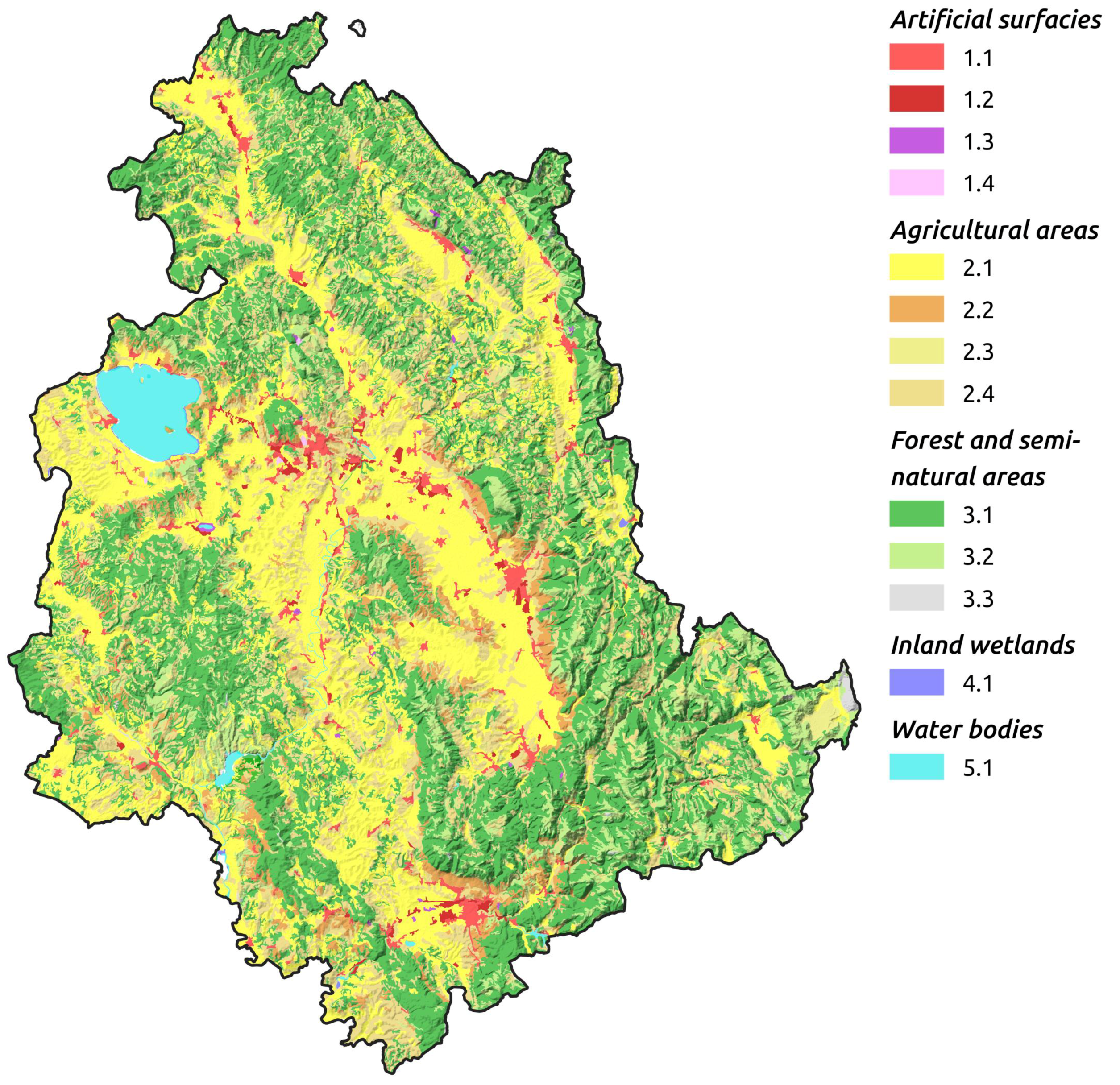
Physiographic characteristics are reflected in land coverage and land use. The Figure 4 shows a land use map derived from CORINE Land Cover data (2nd level), available at http://www.sinanet.isprambiente.it/it/sia-ispra/download-mais/corine-land-cover/corine-land-cover-2012/view.
The natural areas occupy 44.2% of the regional territory and they are mainly located on the mountainous carbonate ridges, placed to the east. On the high hills there is a mixed land use, composed both of natural coverage (forests, shrubs and grass) and of heterogeneous agricultural areas. The hilly and flat areas are widely occupied by agricultural land, occupying over 52.3% of the study area. The most important urban areas and the main infrastructures are found on the widest fluvial valleys.
2.4. Climatic Conditions
For a climate overview of the Umbrian territory we refer to “Relazione sullo Stato dell’Ambiente in Umbria” (i.e., “Report on the State of the Environment in Umbria”), published by the Environment Regional Agency (ARPA) in 2005, available here http://www.arpa.umbria.it/pagine/relazione-sullo-stato-dellambiente-dellumbria.
The document analyzes meteorological data from the bioclimatic and meteoclimatic perspective. In Umbria there are 25 thermometric stations and 78 rain gauges. The analysis has been carried out on four stations, considered representative of the different climatic conditions of the area: Perugia, Gubbio, Terni and Orvieto (see Figure 1 for the location). The data refer to the periods 1956–1999 (Terni and Orvieto), 1956–1997 (Perugia) and 1956–1994 (Gubbio).
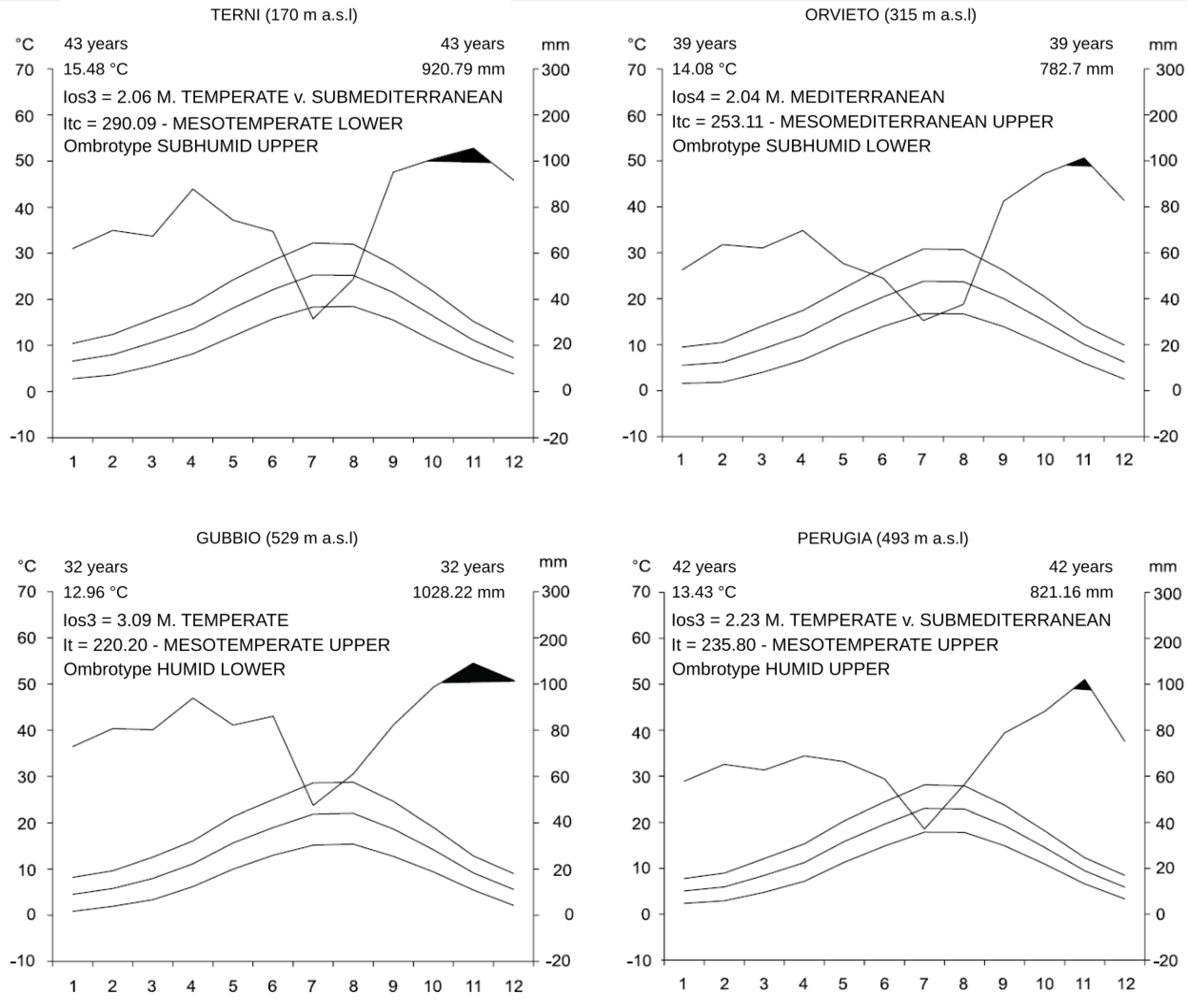
Indices for the definition of the bioclimatic types, as proposed by Rivas-Martínez et al. [22], have been calculated. Table 1 shows the values of the indices, and in Table 2 the bioclimatic types, identified for the four stations considered, are shown. In addition, the ombrothermic diagrams of Walter and Lieth [23] were produced (Figure 5).
Four bioclimatic types have been identified according to the classification proposed by Rivas-Martínez et al. [24]. The climate differences between the various areas are due to the variability of the orographic and physiographic features of the territory (see previous paragraph). The eastern mountainous areas are characterized by consistently higher annual rainfall than the central-western hilly areas. Temperatures values are quite low, in the winter season, in the Apennine area and high (up to 30–35 °C) in summer in the west area, especially in the tectonic valleys.
The analysis of indices trend seems to indicate an evolutionary tendency of the climate towards more arid conditions, although for none of the stations was there observed a substantial change in the bioclimatic category. The report also includes a meteo-climatic analysis of the data. Thermal values for the period 1970–1999 show a tendency to increasing, with slight differences between the various stations, while the pluviometric data show a generalized decreasing.
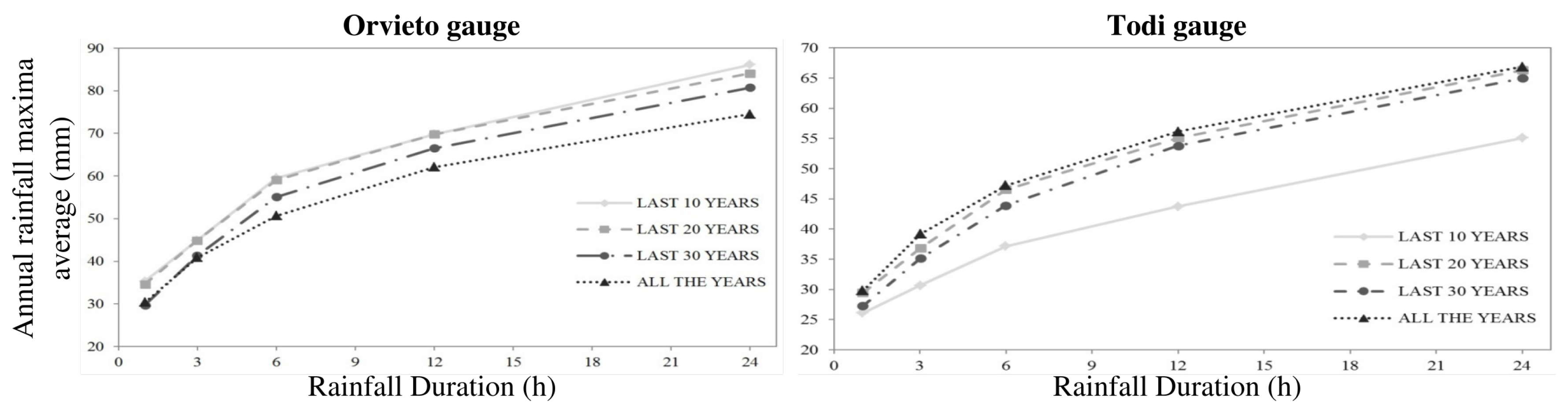
About this topic, the paper of Cifrodelli et al. [25], focused on the influence of climate change on heavy rainfalls in Umbria, is interesting. Three meteorological stations, with longer historical series and less periods of interruption, were chosen: Citta di Castello (north), observation period 1929–2013; Todi (center), observation period 1931–2013 and Orvieto (south-west), observation period 1929–2013 (see Figure 1). The time series were divided into subperiods (last ten years, last twenty years, last thirty years and all the years with recorded measurements) in order to check if frequency and intensity of heavy rainfall changed due to climatic variations.
The data of Città di Castello station did not highlight significant variations in the averages passing from one reference period to another one. The Orvieto station showed a slight increase in maxima averages in the last decade; the trend shows an increasing with the duration (Figure 6). Opposite results were obtained from the Todi series, where the calculated values for the last 10 years are quite lower than all the other ones (Figure 6). The authors concluded that there is not a common trend in the area: the observed variations are generally low and probably caused by local factors (convective air motions or orography) and cannot be related to climate changes.
3. Goal
The web procedure presented in this paper can also be used by “non-experts” to determine the peak flow rate in any specific cross section of the hydrographic network. The method derives from the Flood Estimation Handbook proposed by the Tiber River Basin Authority [18]. The workflow, which originally did not include the use of GIS, has been made possible through the great contribution that geographical instruments offer to territorial analysis. The procedure described in the Flood Estimation Handbook was carried out using the most modern GIS technologies and a web application was developed in order to provide maximum usability and immediacy for obtaining final results. The web application allows the value of the peak flow to be obtained rapidly for a given return period and cross section. Such result can then be used in the fields of hydraulic engineering (in the design phase), administration, territorial planning, geological-hydraulic risk assessment and for problems of fluvial dynamics. The method described is valid exclusively for the area of the Tiber River Basin in the Umbria Region (Central Italy). However, by changing the input parameters, the procedure and the related web application can be applied to any river basin.
4. Method: Procedure for Determining the Peak Flow According to the Flood Estimation Handbook of the Tiber River and Its Proposed Application
The procedure for calculating the peak flow proposed by the Basin Authority of the Tiber River [18] is based on the following simplifications:
- the maximum flood occurs for rainfall duration equal to the run-off time of the contributing basin;
- the peak flow has the same return period as the rain that generated it;
- significant reservoirs are neglected along the hydrographic network: for an assigned hydrograph, the volume of net rain is set as equal to the volume of the peak flow.
The first step in the Flood Estimation Handbook is based on a process of regionalization of rainfall applied to the whole area of Tiber River Basin. Starting from a dataset of maximum rainfall intensity with duration from 1 to 24 h and from 1 to 5 consecutive days, an empirical relationship (intensity duration frequency curve—IDF curve) that correlates rainfall intensity (with a given return period) to duration was calculated for the whole Tiber River Basin. The Tiber River Basin Authority modeled the parameters used in the IDF curve, with respect to a single rainfall station, interpolating them over the entire Tiber River Basin. The Flood Estimation Handbook provides a set of maps defining the parameters a, b, and K for 0–24 h duration and for 1–5 days. The method proceeds according to the following progressive and distinct phases:
- calculation of run-off time;
- calculation of local rainfall depth;
- calculation of areal rainfall depth;
- calculation of infiltration rate and, therefore, net rainfall;
- calculation of peak flow for a specific cross section.
The above phases are illustrated in the following paragraphs.
4.1. Calculation of Run-Off Time
The calculation of run-off time is based on known formulas, extensively validated in the literature. In particular, according to the procedure proposed by the Tiber River Basin Authority, the formulas used are:
- Kirpich, for basins smaller then 10 km:with:
- = run-off time (hours)
- L = main channel length (km)
- = drop in elevation of main channel (m)
- Giandotti, for basins larger than 10 km:with:
- = run-off time (hours)
- S = basin area (km)
- L = main channel length (m)
- H = mean basin elevation (m a.s.l.).
As can be seen, values of the descriptive parameters of the basin morphology are required in both formulas. These parameters (area of the upstream basin, length of the main channel, elevation drop of the main channel, mean basin elevation) are obtained through an automated GIS procedure, as explained in the following chapter.
4.2. Calculation of Local Rainfall
In the process of rainfall regionalization, the Flood Estimation Handbook defines the IDF curve, relating rainfall intensity to duration for a given return period, with the following formulation based on parameters a, b and K:
where:
- h = local rainfall depth in millimetres, lasting D with return period T
- D = duration of rainfall in hours
- RP = return period in years
- = parameters of the IDF curve
- K = coefficient of variation or relative standard deviation
The term , which has local validity, can be expressed as follows:
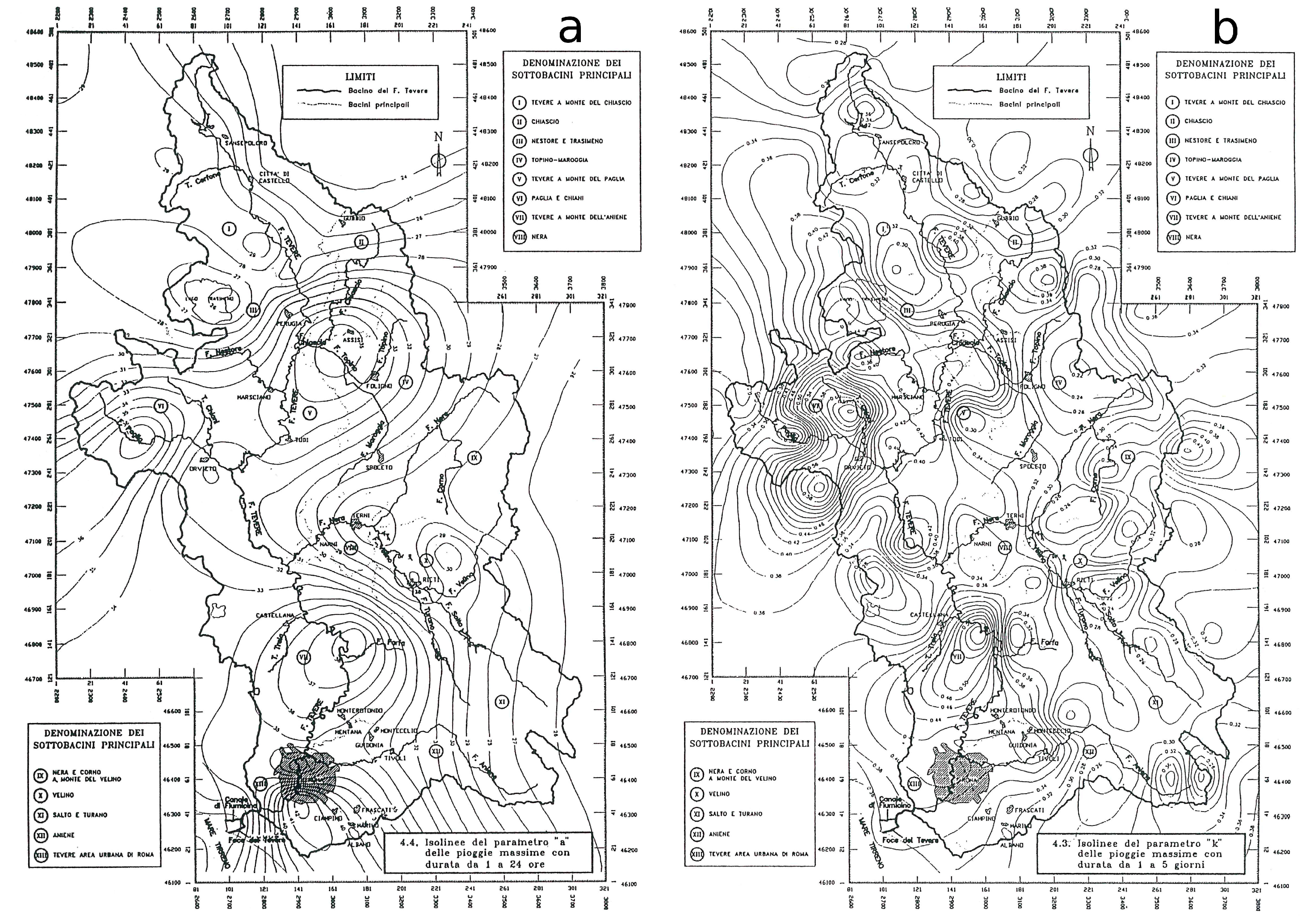
Therefore, knowing the rainfall intensity, the duration, and the return period for a large number of events and for all the gauging stations in the Tiber Basin, isolines were obtained from the Handbook for the three unknown parameters a, b and K (an example is shown in Figure 7), providing maps at the basin scale.
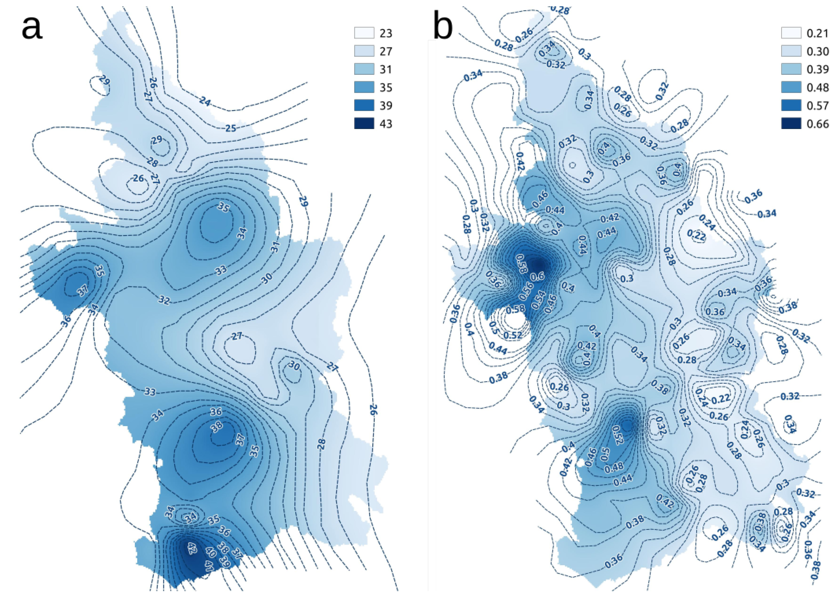
These maps are useful for a quick analysis, because, at any point of the basin, it is possible to obtain values of these three parameters. In particular, in order to develop an automatic GIS procedure, it is necessary to transform the isoline maps into continuous raster maps. The isoline maps were vectorized for a duration of 0–24 h and for a duration of 1–5 days. Then, the vector maps were interpolated using the GRASS GIS module v.surf.rst, which uses the Regularized Spline with Tension [26] obtaining the final raster maps (Figure 8).
4.3. Calculation of Areal Rainfall
Calculation of areal rainfall intensity according to the Flood Estimation Handbook must be carried out using the procedure of the U.S. Weather Bureau that takes into account both rainfall duration and the area affected by it. The formula (valid for rainfall lasting more than 5 min) is as follows:
with:
and where:
- = areal rainfall depth (mm)
- h = local rainfall depth (mm)
- A = basin area (hectares)
- D = rainfall duration (hours)
4.4. Calculation of Net Rainfall: Procedure for Determining the Curve Number
The method defined by the Tiber River Basin Authority states that the net rainfall (the portion of rainfall that reaches a stream channel) is determined by the Curve Number procedure.
The Curve Number (CN) is a dimensionless parameter that defines the characteristic tendency of the basin to runoff, i.e., the fraction of rainfall that does not infiltrate and which reaches the hydrographic network by runoff. The value of the CN decreases as permeability increases from a maximum of 100 to a minimum of 0. It depends on the type of vegetation, type of soil and the initial soil moisture conditions (Antecedent Moisture Condition—AMC). Regarding vegetation coverage, it is necessary to identify the type and density. Regarding soil type, the Soil Conservation Service considers 4 different categories depending on permeability [27].
Normally the reference is to the intermediate moisture condition (AMC II), but it is possible to switch to other moisture conditions using conversion tables. It is necessary to divide the basin into homogeneous areas with assigned CN. The value of the average CN, with respect to the whole basin, is obtained by weighting the values according to the relative areas:
with:
- = ith area
- C = value of CN with respect to the ith area
- A = basin area (m)
To apply the procedure proposed by the Flood Estimation Handbook, it was necessary to evaluate the Curve Number for the entire study area (Umbria Region). CN was not determined for the entire basin of the Tiber River, because only a pedological map of Umbria was available [20]. This map was vectorized and reclassified (Figure 3), attributing to each type of soil (on the base of permeability and texture) the respective class defined by the SCS. The land cover conditions (Figure 4) were determined using data from the European project CORINE Land Cover, which produced a land cover map at 1:100,000 scale for all of Europe. Land use data can be downloaded from the website at: http://www.sinanet.isprambiente.it/it/sia-ispra/download-mais/corine-land-cover/corine-land-cover-2012/view in vector format.
Then, the two layers (soil type and vegetation coverage) were intersected in order to divide the territory of the Umbria Region into homogeneous areas, characterised by a specific soil type and a given class of land use.
Reclassifying the areas previously identified according to Table 3, the CN map was obtained for the entire Umbria Region (Figure 9). The univariate statistics of the CN value for the study area are: mean = 69.0; 10th percentile = 60.5; median = 69.1; 90th percentile = 78.6; standard deviation = 7.8.
Given the areal rainfall () and the average CN of the basin, the net rainfall () is calculated as follows:
with:
and were:
- = net rainfall (mm)
- = areal rainfall (mm)
- = watershed’s maximum retention
- = average CN of the basin
4.5. Calculation of Peak-Flow
Calculation of peak-flow was carried out through a predefined hydrograph shape, following the Gherardelli method, i.e., the triangular hydrogram with rise time equal to descending time. Therefore the peak-flow value is:
with:
- = peak-flow (m/s)
- = net rainfall (mm)
- = run-off time (hours)
- A = basin area (ha)
5. The Calculation Code
Starting from the procedure proposed and illustrated in the previous chapter, a Python code was created for GRASS GIS, able to automate all the above-described steps. This chapter gives details about the calculation code and the features introduced to improve the determination of some parameters and minimise calculation times. The calculation code proceeds by sequential steps:
- Identification of the catchment area;
- Evaluation of the run-off time and identification of the main channel;
- Calculation of the peak-flow;
- Generation of the report.
5.1. Identification of the Catchment Area
For identifying the catchment area, the only input required by the user in the web interface, through a graphic procedure, is the outlet point of the basin and the return period.
To correctly identify the basin upstream from a given cross section, the calculation code find the closest point located exactly on the stream network, since the point provided by the user may not be correctly positioned on it. This point is identified by the r.distance module of GRASS GIS.
To speed up the calculation operations, the raster of the hydrographic network (required as input from r.distance) and the flow direction map (necessary for the next step) have already been calculated for the entire Tiber River Basin, by mean of a Digital Elevation Model. This avoid to reprocess these maps at the request of any user.
We used the DEM provided by the European Copernicus Project called European Digital Elevation Model (EU-DEM), version 1.1. This DEM has a planar resolution of 25 m with a vertical accuracy of 2.9 m, as assessed in https://land.copernicus.eu/pan-european/satellite-derived-products/eu-dem.
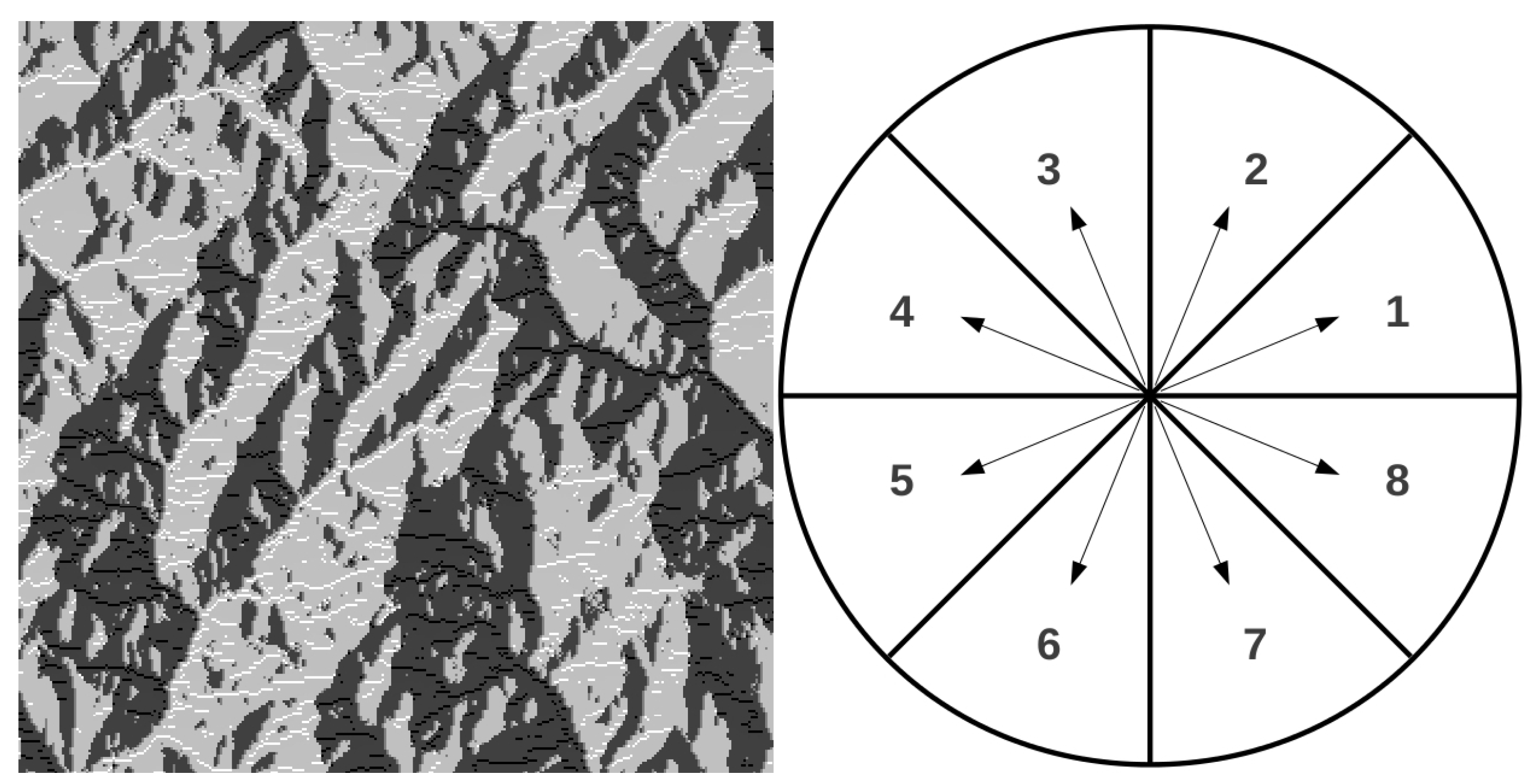
Once the hydrographic network has been calculated and the cross section on the DEM has been identified, the map of the flow direction is used to identify the upstream basin. This map can be obtained directly from the DEM with GRASS GIS, through the r.watershed module: it is a raster map that shows, for each pixel of the examined area, a number that ranges from 1 to 8, indicating the prevailing water flow direction. The numbering starts from the East and proceeds counterclockwise, as shown in Figure 10.
Once the outlet point is correctly located on the hydrographic network, the river basin is delineated using the r.water.outlet module of GRASS GIS.
5.2. Evaluation of Run-Off Time and Identification of the Main Channel
Starting from the hydrographic ordered network, the code selects the maximum order of the stream network and, through a map-algebra operation, extracts the main stream.
The corresponding main channel statistics are derived by the means of the r.stream.stats GRASS GIS module. In particular, the following parameters are calculated:
- length of the main channel
- elevation drop of the main channel
- basin area
- mean basin elevation
- minimum basin elevation
- maximum basin elevation
5.3. Calculation of Peak-Flow
Once the run-off time has been calculated, the IDF parameters (a, b and K) corresponding to the river basin are calculated. Use of the GIS procedure gives a better determination of the aforementioned parameters with respect to the standard procedure proposed by the Flood Estimation Handbook. The Handbook proposes evaluating the IDF parameters with the isoline map at the centroid of the basin; instead, with the GIS procedure, these factors are determined as weighted means of the basin.
Similarly, the Curve Number (CN) is calculated from the raster map previously obtained as the weighted mean value of the basin.
Knowing the values of the a, b, K and CN parameters, the local rainfall (Equation (3)), areal rainfall (Equations (5)–(8)) and net rainfall (Equations (10) and (11)) are then calculated [30]. The peak-flow is calculated with Equation (12). The whole code is freely available at: https://zenodo.org/badge/latestdoi/153136677.
6. Discussion
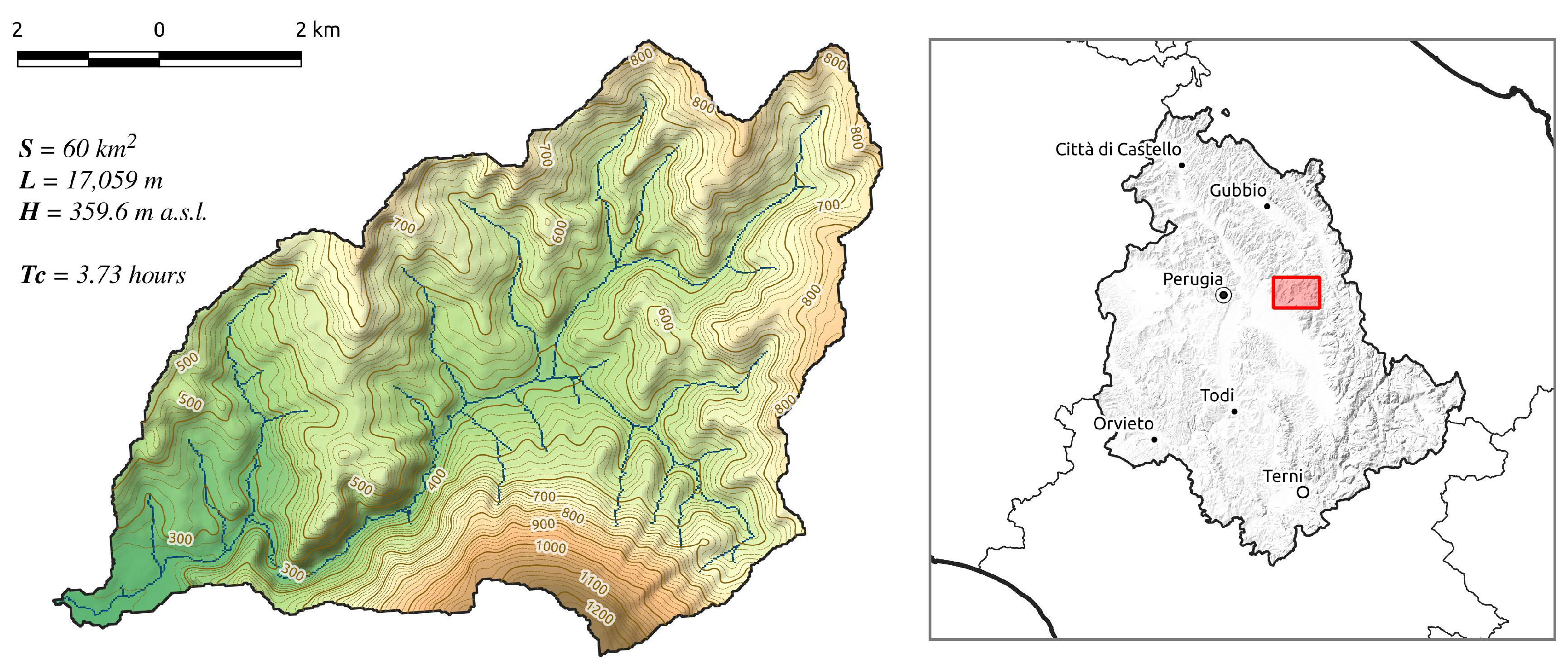
This section is focused on the analysis of the model performance in order to evaluate its sensitivity to DEM resolution/vertical accuracy and to land use / type of soil. Moreover some consideration are presented about the general accuracy of the estimated peak flow. The analysis has been carried out on the Tescio River basin (Figure 11).
6.1. Effects Analysis of the DEM Quality on the Estimated Peak Flow
The DEM is the necessary input data used by the model to calculate the run-off time (). To highlight the relevance of the DEM quality on the final estimated peak flow, 3 different DEMs have been used and compared to the one used in the original procedure (EU-DEM version 1.1).
The selected DEM data, all publicly available in large areas, are:
- EU-DEM version 1.1, covering all Europe—25 m resolution and vertical accuracy of 2.9 m (https://land.copernicus.eu/imagery-in-situ/eu-dem)
- SRTM 1-arc second version V003, covering surfaces that lay between 60 degrees north latitude and 54 degrees south latitude—30 m resolution and declared vertical accuracy of 16 m (https://www2.jpl.nasa.gov/srtm/statistics.html).
- ASTER GDEM Version 2, covering surfaces that lay from 83 degrees north latitude to 83 degrees south—30 m resolution—the ASTER GDEM Validation Team assessed a vertical accuracy of 6.1 m in flat and open areas and 15.1 m in mountainous area largely covered by forest [31].
- TINITALY version 01, covering all Italy—10 m resolution and a vertical accuracy declared by the authors of 3.5 m [32].
A recent study of Elkhrachy [33] asses that the SRTM and ASTER vertical accuracy is better than the declared one: respectively ±5.94 m and ±5.07, using GPS measured elevations, and ±6.87 m and ±7.97 using a topographic map with 1:10,000 scale.
Table 4 reports the results obtained for the Tescio River catchment (area about 60 km—Figure 11), for each DEM. The comparison shows that the peak flow and the run-off time do not vary significantly. This occurs because the four DEMs lead to very similar watershed delineation, and this strongly affects all the morphometric parameters. The TINITALY DEM, which has the highest resolution (10 m), provides an estimated peak flow substantially equal to the values derived from the other DEMs, with lower resolution. The EU-DEM v1.1 is the most suitable for the web application, because it is the most recent and, with a resolution of 25 m, represents a good compromise between reliability of results and computing speed.
6.2. Effects of Curve Number (CN) Value
The CN method is used, in the proposed workflow, to evaluate the net rainfall (i.e., purged of the infiltration fraction). This aspect can be considered a strength of the code, which is able to identify the outlet contributing basin and to analytically determine its average CN, using GIS statistics tools.
The average CN is computed, as described in Section 4.4, starting from a land use map (Figure 4) and a soil type map (Figure 3).
To quantify the CN impact, and indirectly that of land use and soil, the Tescio River basin has been investigated (average CN equal to 81.4—Figure 11). The CN value has been varied, using a modified version of the code, assigning to it the following values: 60.5 (corresponding to the 10th percentile of the CN statistical distribution in the Umbria Region), 69.1 (the real value, next to the 50th percentile) and 78.6 (corresponding to the 90th percentile). The computations results are shown in Table 5.
The Table 5 shows how a proper evaluation of the CN is important to determine the peak flow. In fact we can observe that, keeping the other input parameters unchanged, the peak flow ranges from 81.8 to 207.3 m/s (return period 100 years).
6.3. Evaluation of the Accuracy of Estimated Peak Flow
The River Tiber Basin Authority proposed the procedure here implemented to estimate the peak flow values for non-instrumented small watershed, in order to provide a design flow rate to be used in design of hydraulic works as levee, bridges, etc. The procedure is conceived to be fast and typically overestimates the peak flow compared with more sophisticated ranfall-runoff methods. Di Francesco et al. [34] determinate the peak flow for the Tescio River basin, a small watershed of 60 km (Figure 11) located inside the study area, with a rainfall–runoff model using the real data of three thermo-pluviometric stations. To asses the quality of estimated peak flow, a comparison between the peak flow provided by Di Francesco et al. [34] and the value obtained by the implemented method is reported in Table 6. It appears evident how the differences decrease when the return period increases and the value proposed for return period of 10 years is highly overestimated. In fact, the Flood Estimation Handbook of the Tiber River asses that the proposed procedure should not be used for return period smaller than 50 years.
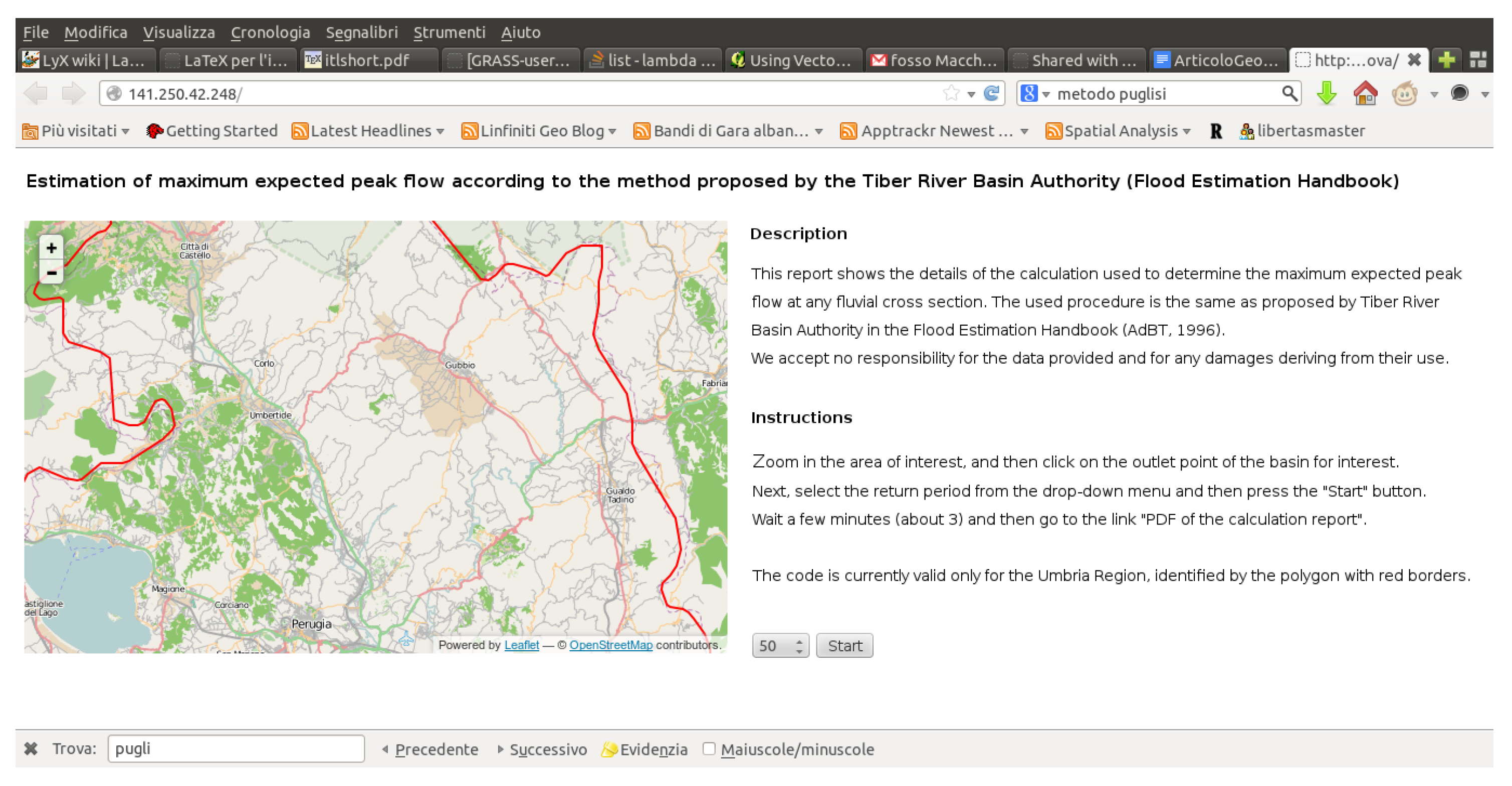
7. Web Tool
The web tool is based on a PyWPS procedure that uses the Python code, described in the previous chapter, called a Leaflet-based web application. The web application shows the user a webmap where the boundary of the Umbria Region is highlighted, since the automatic procedure can be applied only in this area (Figure 12). The user has to select the desired point of the cross section of a stream on the map. A marker is placed on the map to highlight the chosen point. Then the user can select the desired return period from the drop-down menu.
At the end of the procedure the web application generates a PDF report (see Figure 13 where the values of the main parameters are shown. The report can then be downloaded.
The average processing time depends on the size of the catchment area, but in all the tests carried out, 1.5 min have never been exceeded for producing a report. Using Leaflet, the web application can also be used from portable devices such as tablets and smartphones.
8. Conclusions and Future Developments
The paper presents a web application for calculating the flood flow frequency in small basins. The only data input required are outlet coordinates and return period. The algorithm implements the procedure described in the Flood Estimation Handbook proposed by the Tiber River Basin Authority [18]. The aim is provide a tool to estimate peak flow values in non-instrumented small watershed where otherwise it would be not so easy to obtain design flow rate values. Currently there are not many examples of web applications that allow to calculate the flood frequency. Conversely exist several examples of GIS procedures aimed to the same purpose that should be useful to implemented in a WebGIS, as stated by Cheng et al. [15]. The web-application is based on Leaflet libraries (https://leafletjs.com/) for the webmap, and it use PyWPS (http://pywps.org/) as Web Processing Service. The PyWPS calls a GRASS GIS Python script, specifically designed to carry out the computation and generate the final report. All the input data required are constituted by a raster map set (DEM, IDF regional rainfall parameters, land use, type of soil, CN), elaborated by the Authors for the Umbria Region and stored into the computational server. The output analysis shows a low model sensitivity to the DEM resolution; inversely, the Curve Number strongly influences the final result (see Section 6.1 and Section 6.2). Since the method is designed for small basins, it is not trivial obtain measured data with associated return period. Therefore the data modeled by Di Francesco et al. [34] were used to evaluate the quality of the model output. These authors determined designed peak flows (return period 10, 50, 100, 200, 500 years) for the Tescio River basin (60 km watershed located inside the study area) by means of a sophisticated rainfall-runoff model based on the real data of thermo-pluviometric stations. The comparison (see Table 6) shows that the calculated peak flows are overestimated but the overestimation decreases with the increasing of return period. It is considered that the results provided are acceptable for return period equal or greater than 50 years for the following reasons:
- the method is applied to small non-instrumented basins, where hydrological/hydraulic data are not available;
- the peak flow value is used for hydraulic engineering purposes, so a not excessive overestimation ensure higher safety standards.
Therefore, the drop-down menu in the web application does not provide return period below 50 years. Future developments are aimed at improving the graphical interface of the web application and the PDF report. Regarding the Webmap, it is necessary to add more cartographic data, such as a layer of the hydrographic network and the boundary of the Tiber River Basin to allow users to better understand the territorial boundaries in which the calculation code can be used. A map of the basin and the main channel used in the calculation procedure will be included in the calculation report. The map will allow the user to understand if the application has correctly defined the basin and main channel. It is pointed out that the proposed procedure, although valid only for the areas of the Tiber River Basin within the Umbria Region, can be extrapolated to the entire basin, extending the CN map to the Tuscany and Latium Regions. In addition, the method should be able to be applied to any river basin, once the basic parameters required by the code have been determined (in this case not only CN, but also the a, b and K coefficients).
Author Contributions
P.D.R. implemented the python code and the web-application. A.F. designed the code algorithm, the web-map and the report; checked the output. All authors wrote the paper.
Funding
This research was funded by Umbria Region (Italy), grant number DD:4794/2011.
Acknowledgments
This paper is based on research carried out as part of the innovation research project titled “Evaluation of the risk conditions due to landslide dams in Umbria. Identification on a regional scale of situations characterised by different hazard”—Coordinator: Corrado Cencetti’. We would like to thank the Umbria Region for funding the research.
Conflicts of Interest
The authors declare no conflict of interest.
References
- Rodríguez-Iturbe, I.; Valdés, J.B. The geomorphologic structure of hydrologic response. Water Resour. Res. 1979, 15, 1409–1420. [Google Scholar] [CrossRef] [Green Version]
- Gupta, V.K.; Waymire, E.; Wang, C.T. A representation of an instantaneous unit hydrograph from geomorphology. Water Resour. Res. 1980, 16, 855–862. [Google Scholar] [CrossRef]
- Rodríguez-Iturbe, I.; González-Sanabria, M.; Bras, R.L. A geomorphoclimatic theory of the instantaneous unit hydrograph. Water Resour. Res. 1982, 18, 877–886. [Google Scholar] [CrossRef]
- Giannoni, F.; Roth, G.; Rudari, R. A procedure for drainage network identification from geomorphology and its application to the prediction of the hydrologic response. Adv. Water Resour. 2005, 28, 567–581. [Google Scholar] [CrossRef]
- Kumar, R.; Chatterjee, C.; Singh, R.D.; Lohani, A.K.; Kumar, S. Runoff estimation for an ungauged catchment using geomorphological instantaneous unit hydrograph (GIUH) models. Hydrol. Process. 2007, 21, 1829–1840. [Google Scholar] [CrossRef]
- Noto, L.V.; La Loggia, G. Derivation of a Distributed Unit Hydrograph Integrating GIS and Remote Sensing. J. Hydrol. Eng. 2007, 12, 639–650. [Google Scholar] [CrossRef]
- Brocca, L.; Melone, F.; Moramarco, T. Modellistica afflussi-deflussi di tipo continuo per la previsione delle piene su bacini dell’Alto-Medio Tevere. In Atti del XXXII Convegno Nazionale di Idraulica e Costruzioni Idrauliche; Farina: Palermo, Italy, 2010. [Google Scholar]
- Petroselli, A.; Grimaldi, S.; Alonso, G.; Nardi, F. Modelli afflussi deflussi per piccoli bacini idrografici non strumentati. In Atti del XXXII Convegno Nazionale di Idraulica e Costruzioni Idrauliche; Farina: Palermo, Italy, 2010. [Google Scholar]
- Grimaldi, S.; Petroselli, A.; Nardi, F.; Tauro, F. Analisi critica dei metodi di stima del tempo di corrivazione. In Atti del XXXII Convegno Nazionale di Idraulica e Costruzioni Idrauliche; Farina: Palermo, Italy, 2010. [Google Scholar]
- Domniţa, M.; Crăciun, I.; Haidu, I.; Magyari-Sáska, Z. GIS used for determination of the maximum discharge in very small basins (under 2 km2). WSEAS Trans. Environ. Dev. 2010, 6, 468–477. [Google Scholar]
- David, V.; Davidova, T. Methodology for flood frequency estimations in small catchments. Nat. Hazards Earth Syst. Sci. 2014, 14, 2655–2669. [Google Scholar] [CrossRef] [Green Version]
- Teresneu, C.C. Using gis for the determination of peak discharge in a small forested watershed. Bull. Transilv. Univ. Brasov. For. Wood Ind. Agric. Food Eng. Ser. II 2013, 6, 69. [Google Scholar]
- Dang, A.T.N.; Kumar, L. Application of remote sensing and GIS-based hydrological modelling for flood risk analysis: A case study of District 8, Ho Chi Minh city, Vietnam. Geomat. Nat. Hazards Risk 2017, 8, 1792–1811. [Google Scholar] [CrossRef]
- Uddin, K.; Gurung, D.R.; Giriraj, A.; Shrestha, B. Application of Remote Sensing and GIS for Flood Hazard Management: A Case Study from Sindh Province, Pakistan. Am. J. Geogr. Inf. Syst. 2013, 2, 1–5. [Google Scholar]
- Cheng, Q.; Ko, C.; Yuan, Y.; Ge, Y.; Zhang, S. GIS modeling for predicting river runoff volume in ungauged drainages in the Greater Toronto Area, Canada. Comput. Geosci. 2006, 32, 1108–1119. [Google Scholar] [CrossRef]
- Kulkarni, A.; Mohanty, J.; Eldho, T.; Rao, E.; Mohan, B. A web GIS based integrated flood assessment modeling tool for coastal urban watersheds. Comput. Geosci. 2014, 64, 7–14. [Google Scholar] [CrossRef]
- Eldho, T.I.; Zope, P.E.; Kulkarni, A.T. Chapter 12—Urban Flood Management in Coastal Regions Using Numerical Simulation and Geographic Information System. In Integrating Disaster Science and Management; Samui, P., Kim, D., Ghosh, C., Eds.; Elsevier: Amsterdam, The Netherlands, 2018; pp. 205–219. [Google Scholar]
- Autorità di Bacino del Fiume Tevere. Quaderno idrologico del Fiume Tevere. Tevere 1996, 1, 64. [Google Scholar]
- Pantaloni, M.; Bonomo, R.; Capotorti, F.; Compagnoni, B.; D’Ambrogi, C.; Di Stefano, R.; Galluzzo, F.; Graziano, R.; Martarelli, L.; Letizia Pampaloni, M.; et al. La nuova Carta Geologica d’Italia alla scala 1:500,000. Memorie Descrittive Carta Geologica d’Italia 2006, 1, 113–114. [Google Scholar]
- Giovagnotti, C.; Calandra, R.; Leccese, A.; Giovagnotti, E. I Paesaggi Pedologici e la Carta dei Suoli del l’Umbria; Camera di Commercio, Industria, Artigianato e Agricoltura di Perugia: Todi, Italy, 2003. [Google Scholar]
- Soil Science Division Staff. Soil Survey Manual; Handbook 18; Ditzler, C., Scheffe, K., Monger, H.C., Eds.; United States Department of Agriculture: Washington, DC, USA, 2017. [Google Scholar]
- Rivas-Martínez, S.; Rivas-Saenz, S.; Penas, A. Worldwide Bioclimatic Classification System; Backhuys Pub.: Kerkwerve, The Netherlands, 2002. [Google Scholar]
- Walter, H.; Lieth, H. Klimadiagramm-Weltatlas [World Climate Diagram]; Gustav Fischer: Jena, Germany, 1960. [Google Scholar]
- Rivas-Martínez, S.; Sánchez-Mata, D.; Costa, M. North American boreal and western temperate forest vegetation. Itinera Geobotanica 1999, 12, 5–316. [Google Scholar]
- Cifrodelli, M.; Corradini, C.; Morbidelli, R.; Saltalippi, C.; Flammini, A. The Influence of Climate Change on Heavy Rainfalls in Central Italy. Procedia Earth Planet. Sci. 2015, 15, 694–701. [Google Scholar] [CrossRef]
- Mitášová, H.; Mitáš, L. Interpolation by regularized spline with tension: I. Theory and implementation. Math. Geol. 1993, 25, 641–655. [Google Scholar] [CrossRef] [Green Version]
- Mockus, V. National Engineering Handbook Section 4, Hydrology; Technical Report; U.S. Department of Agriculture, Soil Conservation Service: Washington, DC, USA, 1969.
- Horton, R.E. Erosional Development of stream and their drainage basins; Hydrophysical approach to quantitative morphology. GSA Bull. 1945, 56, 275–370. [Google Scholar] [CrossRef]
- Jasiewicz, J.; Metz, M. A new GRASS GIS toolkit for Hortonian analysis of drainage networks. Comput. Geosci. 2011, 37, 1162–1173. [Google Scholar] [CrossRef]
- Cronshey, R. Urban Hydrology for Small Watersheds, 2nd ed.; Technical Report; U.S. Department of Agriculture, Soil Conservation Service, Engineering Division: Washington, DC, USA, 1986.
- Tachikawa, T.; Kaku, M.; Iwasaki, A.; Gesch, D.B.; Oimoen, M.J.; Zhang, Z.; Danielson, J.J.; Krieger, T.; Curtis, B.; Haase, J.; et al. ASTER Global Digital Elevation Model Version 2—Summary of Validation Results; Report; NASA: Washington, DC, USA, 2011; Available online: https://ssl.jspacesystems.or.jp/library/archives/ersdac/GDEM/ver2Validation/Summary_GDEM2_validation_report_final.pdf (accessed on 18 December 2018).
- Tarquini, S.; Isola, I.; Favalli, M.; Mazzarini, F.; Bisson, M.; Pareschi, M.T.; Boschi, E. TINITALY/01: A new Triangular Irregular Network of Italy. Ann. Geophys. 2007, 50, 407–425. [Google Scholar] [CrossRef]
- Elkhrachy, I. Vertical accuracy assessment for SRTM and ASTER Digital Elevation Models: A case study of Najran city, Saudi Arabia. Ain Shams Eng. J. 2017. [Google Scholar] [CrossRef]
- Di Francesco, S.; Biscarini, C.; Manciola, P. Characterization of a Flood Event through a Sediment Analysis: The Tescio River Case Study. Water 2016, 8, 308. [Google Scholar] [CrossRef]
Figure 1.
Tiber River Basin in the Umbrian area, in central Italy. The hashed polygon (1) represent the Tiber River Basin while the yellow polygon (2) represent the Umbria Region.
Figure 1.
Tiber River Basin in the Umbrian area, in central Italy. The hashed polygon (1) represent the Tiber River Basin while the yellow polygon (2) represent the Umbria Region.

Figure 2.
Geolithological map of Umbria Region. 1 = Carbonate marine formations, distinguished in neritic and carbonate platform facies sequence (a) and in pelagic facies sequence (b); 2 = Siliciclastic marine formations (flysch); 3 = Unconsolidated continental deposits of lacustrine and fluvial-lacustrin facies; 4 = Recent and terraced alluvial deposits; 5 = Unconsolidated marine deposits, distinguished in coastal/deltaic plain sequence (a) and in deeper marine environment sequence (b); 6 = Volcanic rocks. Data source: Geological map of Italy (1: 500,000 scale), by Geological Service of Italy [19].

Figure 3.
Pedological map of Umbria Region. Soils are defined using the ternary diagram of the USDA soil texture classification [21]: Cl = Clay; Si-Cl = Silty clay; Cl-Lo = Clay loam; Lo = Loam; Sa-Lo = Sandy Loam, Lo-Sa = Loamy sand; Sa = Sand; Si-Cl-Lo = Silty clay loam; Si-Lo = Silt loam. Data source: Soils map of Umbria [20].

Figure 4.
Land use map of Umbria Region. 1.1 = Urban fabric; 1.2 = Industrial, commercial or transport units; 1.3 = Mines, dumps and construction sites; 1.4 = Artificial, non agricultural, vegetated areas; 2.1 = Agricultural areas; 2.2 = Permanent crops; 2.3 = Pastures; 2.4 = heterogeneous agricultural areas; 3.1 = Forests; 3.2 = Shrubs and/or Herbaceous vegetation associations; 3.3 = Open space with little or no vegetation; 4.1 = Inland wetlands; 5.1 = Inland waters. Data source: CORINE Land Cover (2nd level), at http://www.sinanet.isprambiente.it/it/sia-ispra/download-mais/corine-land-cover/corine-land-cover-2012/view.

Figure 5.
Ombrothermic diagrams for the selected stations. Source: Report on the state of the environment in Umbria, available at http://www.arpa.umbria.it/pagine/relazione-sullo-stato-dellambiente-dellumbria.
Figure 5.
Ombrothermic diagrams for the selected stations. Source: Report on the state of the environment in Umbria, available at http://www.arpa.umbria.it/pagine/relazione-sullo-stato-dellambiente-dellumbria.

Figure 6.
Annual rainfall maxima averages for different durations and over different time periods for the Orvieto and Todi data series [25].
Figure 6.
Annual rainfall maxima averages for different durations and over different time periods for the Orvieto and Todi data series [25].

Figure 7.
Examples of the maps of the isolines for the a (a) and K (b) parameters taken from the Flood Estimation Handbook of the Tiber River Basin Authority.
Figure 7.
Examples of the maps of the isolines for the a (a) and K (b) parameters taken from the Flood Estimation Handbook of the Tiber River Basin Authority.

Figure 8.
Examples of the maps obtained by interpolating the isolines shown in Figure 7. (a) shows the value of a parameter of IDF related to 0–24 h of duration; (b) shows the value of K parameter of IDF related to 1–5 days of duration
Figure 8.
Examples of the maps obtained by interpolating the isolines shown in Figure 7. (a) shows the value of a parameter of IDF related to 0–24 h of duration; (b) shows the value of K parameter of IDF related to 1–5 days of duration

Figure 9.
Curve Number map for the territory of the Umbria Region. In legend the values corresponds to the CN.
Figure 9.
Curve Number map for the territory of the Umbria Region. In legend the values corresponds to the CN.

Figure 10.
Example of a map of drainage directions (left) and procedure for assigning the outflow direction from cell to cell (right).
Figure 10.
Example of a map of drainage directions (left) and procedure for assigning the outflow direction from cell to cell (right).

Figure 11.
Main morphological parameters for the Tescio River basin. S = basin area; L = main channel length; H = mean basin elevation; = run-off time.
Figure 11.
Main morphological parameters for the Tescio River basin. S = basin area; L = main channel length; H = mean basin elevation; = run-off time.

Figure 12.
Web interface for evaluating the expected peak-flow rate, at every point of the hydrographic network of the Umbria Region, using the procedure of the Flood Estimation Handbook of the Tiber River.
Figure 12.
Web interface for evaluating the expected peak-flow rate, at every point of the hydrographic network of the Umbria Region, using the procedure of the Flood Estimation Handbook of the Tiber River.

Figure 13.
Example of report.


Table 1.
Main bioclimatic indices. Ic = Continentality index; Io = Annual ombrothermic index; Ios1 = Ombrothermic index of the warmest summer month; Ios2 = Ombrothermic index of the warmest summer bimester; Ios3 = Ombrothermic index of summer; Ios4 = Ombrothermic index of summer (June + July + August) and the previous month (May); It = Thermicity index; Itc = Compensated thermicity index. Source: Report on the state of the environment in Umbria, available at http://www.arpa.umbria.it/pagine/relazione-sullo-stato-dellambiente-dellumbria.
| Orvieto | Terni | Perugia | Gubbio | |
|---|---|---|---|---|
| Observed years | 43 | 39 | 39 | 32 |
| Ic | 18.58 | 18.27 | 17.91 | 17.53 |
| Io | 4.96 | 4.63 | 5.09 | 6.61 |
| Ios1 | 1.25 | 1.28 | 1.61 | 2.77 |
| Ios2 | 1.59 | 1.43 | 2.04 | 2.47 |
| Ios3 | 2.06 | 1.72 | 2.33 | 3.09 |
| Ios4 | 2.04 | |||
| It | 286.70 | 251.75 | 235.80 | 220.20 |
| Itc | 290.09 | 253.11 |
Table 2.
Main bioclimatic types for the selected stations. Source: Report on the state of the environment in Umbria, available at http://www.arpa.umbria.it/pagine/relazione-sullo-stato-dellambiente-dellumbria.
Table 2.
Main bioclimatic types for the selected stations. Source: Report on the state of the environment in Umbria, available at http://www.arpa.umbria.it/pagine/relazione-sullo-stato-dellambiente-dellumbria.
| Orvieto | Terni | Perugia | Gubbio | |
|---|---|---|---|---|
| Macrobioclimate | mediterranean | temperate | temperate | temperate |
| Bioclimate | oceanic | oceanic | oceanic | oceanic |
| semicontinental | semicontinental | |||
| Bioclimatic variant | submediterranean | submediterranean | ||
| Thermotype | mesomediterranean | mesotemperate | mesotemperate | mesotemperate |
| lower | upper | upper | ||
| Ombrotype | subhumid lower | subhumid upper | subhumid upper | humid lower |
Table 3.
Correlations used for assigning the CN value.
| 1st Level CORINE Land Cover | 2nd Level CORINE Land Cover | 3rd Level CORINE Land Cover | Soil Permeability | |||
|---|---|---|---|---|---|---|
| A | B | C | D | |||
| Artificial Land Cover | Urbanized Areas | Continuous urban fabric | 89 | 92 | 94 | 95 |
| Discontinuous urban fabric | 77 | 85 | 90 | 92 | ||
| Industrial or commercial units, road and rail networks | Industrial or commercial areas | 81 | 88 | 91 | 93 | |
| Road and rail networks and accessory spaces | 98 | 98 | 98 | 98 | ||
| Airports | 98 | 98 | 98 | 98 | ||
| Mineral extraction sites, dumps, construction sites | Mineral extraction sites | 51 | 68 | 79 | 84 | |
| Construction sites | 51 | 68 | 79 | 84 | ||
| Green urban areas | Sport and leisure facilities | 39 | 61 | 74 | 80 | |
| Land mainly occupied by agriculture, with significant areas of natural vegetation | Arable land | Non-irrigated arable land | 72 | 81 | 88 | 91 |
| Permanently irrigated land | Vineyards | 72 | 81 | 88 | 91 | |
| Olive groves | 72 | 81 | 88 | 91 | ||
| Natural grasslands | Natural grasslands | 30 | 58 | 71 | 78 | |
| Heterogeneous agricultural areas | Annual crops associated with permanent crops | 62 | 71 | 78 | 81 | |
| Cropping systems with permanent particles | 62 | 71 | 78 | 81 | ||
| Land mainly occupied by agriculture, with significant areas of natural vegetation | 62 | 71 | 78 | 81 | ||
| Wooded territories and semi-natural environments | Forestry areas | Broad-leaved forest | 25 | 55 | 70 | 77 |
| Coniferous forest | 45 | 66 | 77 | 83 | ||
| Mixed forest | 25 | 55 | 70 | 77 | ||
| Areas characterized by shrub and/or herbaceous vegetation | Pastures | 39 | 61 | 74 | 80 | |
| Moors and heathland | 39 | 61 | 74 | 80 | ||
| Sclerophyllous vegetation | 39 | 61 | 74 | 80 | ||
| Transitional woodland-shrub | 39 | 61 | 74 | 80 | ||
| Open areas with sparse or absent vegetation | Beaches, dunes, sands | 49 | 69 | 79 | 84 | |
| Bare rocks | 49 | 69 | 79 | 84 | ||
| Sparsely vegetated areas | 49 | 69 | 79 | 84 | ||
| Wetlands | Inland wetlands | Inland marshes | 100 | 100 | 100 | 100 |
| Water bodies | Continental waters | Water courses | 100 | 100 | 100 | 100 |
| Water basins | 100 | 100 | 100 | 100 | ||
Table 4.
Comparison between the peak flow output and some significant parameters obtained from the selected DEM. Res. = cellsize dimension; Vert. Acc. = vertical accuracy; S = basin area; L = main channel length; H = mean basin elevation; = run-off time; = peak flow; diff. = difference in percentage compared with EU-DEM.
| Res. | Vert. Acc. | S | L | H | ||||
|---|---|---|---|---|---|---|---|---|
| (m) | (m) | (ha) | (m) | (m a.s.l.) | (hours) | (m/s) | diff. (%) | |
| EU-DEM | 25 | 2.9 | 6024.74 | 17058.9 | 359.6 | 3.73 | 134.73 | / |
| SRTM | 30 | 16 | 6014.08 | 17126.5 | 357.4 | 3.75 | 134.15 | −0.4 |
| ASTER GDEM | 30 | 6.1 to 15 | 6006.90 | 15978.2 | 354.23 | 3.65 | 135.71 | 0.7 |
| TINITALY | 10 | 3.5 | 6092.81 | 17369.7 | 355.59 | 3.80 | 135.07 | 0.3 |
Table 5.
Computational results (return period 100 years) for three CN values, corresponding to the 10th, 50th and 90th percentile of the CN statistical distribution in the Umbria Region.
Table 5.
Computational results (return period 100 years) for three CN values, corresponding to the 10th, 50th and 90th percentile of the CN statistical distribution in the Umbria Region.
| Average CN | Basin Area | Local Rainfall | Areal Rainfall | Net Rainfall | Peak Flow |
|---|---|---|---|---|---|
| (ha) | (mm) | (mm) | (mm) | (m/s) | |
| 60.5 | 6025 | 104.4 | 98.1 | 18.3 | 81.8 |
| 69.1 | 6025 | 104.4 | 98.1 | 30.1 | 134.7 |
| 78.6 | 6025 | 104.4 | 98.1 | 46.3 | 207.3 |
Table 6.
Comparison, for different return period, between peak flows calculated by Di Francesco et al. model [34] and the peak flows calculated by the proposed model.
Table 6.
Comparison, for different return period, between peak flows calculated by Di Francesco et al. model [34] and the peak flows calculated by the proposed model.
| Years | T = 10 | T = 50 | T = 100 | T = 200 | T = 500 |
|---|---|---|---|---|---|
| Reference peak flow (m/s) | 12.52 | 88.04 | 116.86 | 148.46 | 191.98 |
| Modelled peak flow (m/s) | 53.43 | 108.23 | 134.73 | 162.69 | 201.60 |
| Difference (m/s) | 40.91 | 20.19 | 17.87 | 14.23 | 9.62 |
| Difference (%) | 326.8 | 22.9 | 15.3 | 9.6 | 5.0 |
© 2018 by the authors. Licensee MDPI, Basel, Switzerland. This article is an open access article distributed under the terms and conditions of the Creative Commons Attribution (CC BY) license (http://creativecommons.org/licenses/by/4.0/).
Share and Cite
MDPI and ACS Style
De Rosa, P.; Fredduzzi, A.; Minelli, A.; Cencetti, C. Automatic Web Procedure for Calculating Flood Flow Frequency. Water 2019, 11, 14. https://doi.org/10.3390/w11010014
AMA Style
De Rosa P, Fredduzzi A, Minelli A, Cencetti C. Automatic Web Procedure for Calculating Flood Flow Frequency. Water. 2019; 11(1):14. https://doi.org/10.3390/w11010014
Chicago/Turabian StyleDe Rosa, Pierluigi, Andrea Fredduzzi, Annalisa Minelli, and Corrado Cencetti. 2019. "Automatic Web Procedure for Calculating Flood Flow Frequency" Water 11, no. 1: 14. https://doi.org/10.3390/w11010014
Note that from the first issue of 2016, this journal uses article numbers instead of page numbers. See further details here.