Three-Dimensional Temperature Field Change in the South China Sea during Typhoon Kai-Tak (1213) Based on a Fully Coupled Atmosphere–Wave–Ocean Model

Abstract

Studying the sea–air interaction between the upper ocean and typhoons is crucial to improve our understanding of heat and momentum exchange between the atmosphere and the ocean. There is a strong heat flux exchange between the atmosphere and the ocean during the impact of a typhoon, and the physical fields, such as the wind field, wave field, flow field, and SST field, also interact with each other. A fully coupled Atmosphere–Wave–Ocean model in the South China Sea was established by the mesoscale atmospheric model WRF, wave model SWAN, and the regional ocean model ROMS based on the COAWST model system. Typhoon Kai-tak was simulated using this fully coupled model and some other coupled schemes. In this paper, the variation of sea surface temperature (SST) and ocean subsurface temperature caused by Typhoon Kai-tak is analyzed by the fully coupled model, and the basic characteristics of the response of the upper ocean to the typhoon are given. The simulation results demonstrate that the fully coupled WRF-SWAN-ROMS model shows that the typhoon passes through the sea with obvious cooling. In the cold eddy region, the sea surface temperature cools 4 to 5 °C, and the cooling zone is concentrated on the right side of the track. The change of sea surface temperature lags more than 12 h behind the change of sea surface height. The decrease of SST on the left side of the track was relatively small: ranging from 1.5 to 2.5 °C. The disturbance of typhoon causes the subsurface water to surge to the surface, changes the temperature distribution of the surface, and causes the mixing layer to deepen about 40 m to 60 m. The simulation results reveal the temporal and spatial distribution of sea temperature and mixed layer depth. The sea surface temperature field has an asymmetrical distribution in space and has a lag in time. The heat exchange at the air–sea interface is very strong under the influence of the typhoon. The heat exchange between the air and sea is divided into latent heat and sensible heat, and the latent heat generated by water vapor evaporation plays a dominant role in the heat exchange at the air–sea interface, which shows that the heat carried by the vaporization of the sea surface is one of the important factors for the decrease of sea temperature under the influence of the typhoon.

1. Introduction

Tropical cyclones are some of the most destructive natural disasters, which often bring huge losses to people’s life and property. The Northwest Pacific and the South China Sea regions are the birthplaces of most monsoons and typhoons and are important channels for the generation and transmission of water vapor [1,2,3,4,5]. With an increase in sea surface temperature (SST), the total number of tropical cyclones in the North Pacific, Indian Ocean, and southwest Pacific Ocean decreases, and the cyclone development period shortens, but the number and proportion of tropical cyclones reaching super typhoon intensity increases greatly [6,7].

The influence of a typhoon on a region is often not only a heavy wind disaster. At the same time, the heavy rain, extreme waves, storm surges, and coastal inundation that are produced will also have a huge impact on the region, which will result in the formation of a typhoon disaster chain [8,9,10,11]. Therefore, studying the movement mechanism of typhoon, accurately forecasting the influence of typhoon and reducing storm surge disasters have important social value for the protection of national economic development and people’s lives and property safety [12,13].

In the study of air–sea interaction, the response of the upper ocean to typhoons is a hot topic [14]. Studying the interaction between the upper ocean and the typhoons is crucial to improve our understanding of heat and momentum exchange between the ocean and the atmosphere. In recent years, the upper ocean responses to typhoons have received considerable attention. Typhoon transit can cause ocean mixing and upwelling, and sea surface cooling is the main feature [15,16,17]. The cooling caused by a typhoon is mainly related to the intensity, propagation speed of the typhoon, and the ocean condition before typhoon arrival, such as the location of cold vortices, the thermodynamic structure of the upper ocean, the position of the 26 °C isotherm, etc.

Cyclonic wind stress results in the upwelling of sea water in the center of the path, the decrease of sea surface temperature, and the heat transfer from the surface to the atmosphere. Strong winds cause turbulent mixing of the ocean, entraining cold water from the lower layer into the mixing layer, resulting in cooling of the upper sea water and deepening of the mixing layer [18,19,20,21]. Inclusive mixing disturbances cause 85% of irreversible ocean heat to enter the atmosphere; direct air–sea interaction plays a minor role in surface cooling. Mixed layer plays an important role in sea surface cooling [22,23,24]. After typhoon transit, the ocean response is mostly the internal nonlocal baroclinic process caused by wind stress. In baroclinic driving stage, the flow of mixing layer 1 m/s is induced by vertical mixing, and the flow of near-inertial oscillation frequency wave into thermocline, which lasts for 5–10 days. The barotropic driving process usually results in geostrophic currents and associated sea surface height changes.

Using the observed data to study the ocean response to typhoons is a common research method. However, due to the severe weather conditions during the transit of tropical cyclones, it is very difficult to obtain fixed-point observation data. There is a strong mass transport, energy exchange, and interaction between the atmosphere and the ocean during a typhoon process [25,26]. The physical fields such as the wind field, flow field, and wave field influence each other and restrict each other. The forcing effect of the atmosphere on the ocean mainly includes wind stress, pressure, heat flux, and solar radiation on the sea surface. At the same time, the upper ocean responds to the atmospheric effects, and its response results in atmospheric dynamics processes. The role of the oceans in the atmosphere mainly includes two aspects. First, changes in the sea surface temperature (SST) lead to changes in the sea surface heat flux, which affect the movement of the atmosphere. Second, changes in the sea surface flow field cause the wind stress at the bottom of the atmosphere to change, and affect the atmosphere movement structure [27]. In summary, during the evolution of storm surge induced by typhoon there are many influencing factors, including the influence of different spatial and temporal scales and different physical factors, such as wind speed, air pressure, runoff, wave, astronomical tide, and others, which make it difficult to accurately simulate storm surges [28,29,30,31].

In this study, a full coupled Atmosphere–Wave–Ocean model is used to simulate the temperature and salinity changes in the upper ocean under the influence of typhoon. The coupled WRF-SWAN-ROMS model in the South China Sea has been established by the model coupling toolkit (MCT), the mesoscale atmospheric model WRF, the wave model SWAN, and the regional ocean model ROMS, which is based on the COAWST model system in this study. The typhoon wind and pressure field, typhoon waves and storm surge under the influence of actual Typhoon Kai-tak were simulated based on this coupled model and some other coupled schemes. The characteristics of atmospheric, wave, and oceanic results in the South China Sea under the influence of typhoon were calculated. The characteristics of thermohaline structures in the South China Sea during Typhoon Kai-tak were analyzed in this study. The response of the upper ocean during the Typhoon Kai-tak is studied to reveal the characteristics of SST, SSA, and subsurface temperature changes.

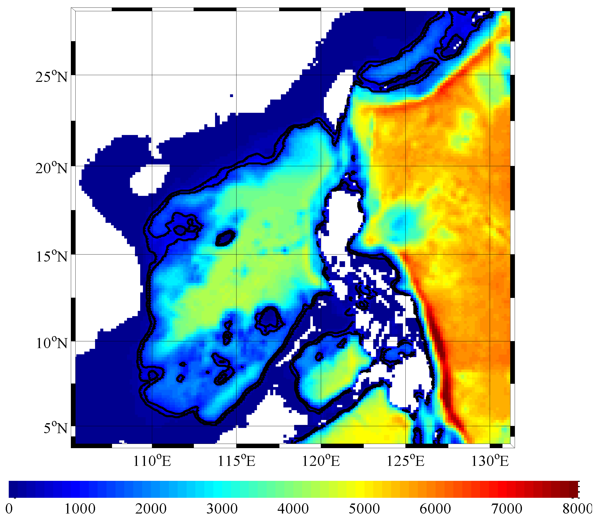
2. Study Site and Implementation of COAWST

2.1. Numerical Tools: The COAWST Model System

The COAWST model system was presented and developed by Warner et al. [32,33] which included a mesoscale atmospheric model WRF, a wave generation and propagation model SWAN and a regional ocean model ROMS. The model coupled toolkit (MCT) as the coupler is used to exchange physical information between different models.

2.1.1. Physical Exchange in the Coupled Model

The fully coupled Atmosphere–Wave–Ocean model of the South China Sea was established based on the WRF-SWAN-ROMS model and the MCT coupler in this study. The following physical exchanges occurred between the models.

(1)

WRF2SWAN: 10-m wind speed (U10, V10);

(2)

SWAN2WRF: sea surface roughness simulated by wave height (Hs), wave length (Len.), and wave period (Per.) using Formulas (1) and (2);

(3)

WRF2ROMS: sea surface stress ($\tau$), surface pressure, net heat fluxes, sensible heat flux, latent heat flux, shortwave radiation flux, and longwave radiation flux;

(4)

ROMS2WRF: sea surface temperature (SST);

(5)

SWAN2ROMS: wave height (Hs), wave direction (Dir.), wave length (Len.), wave period (Per.), and other wave parameters, as well as bottom orbital velocity;

(6)

ROMS2SWAN: topography, zeta, and depth-average velocity (u_a and v_a).

Regarding the calculation of sea surface roughness, it can be divided into two cases: with and without wave influence. Without wave influence, sea surface roughness is computed in WRF is based on the Charnock [34] relation of roughness length to wind stress:

$$z_0=z_{Ch}\frac{u_{*}^2}{g}$$

(1)

where, $z_0$ is the roughness length, $z_{Ch}$ is the Charnock number (a dimensionless number of 0.018), $u_{*}^{}$ is the friction velocity (m/s), and $g$ is the gravity acceleration (9.8 m/s²).

With the wave actions, the sea surface roughness was calculated by comparison of intensity and wave height, the Taylor and Yelland (2001) [35] method was selected in this study.

$$\frac{z_0}{H_s}=A_1{\left(\frac{H_s}{L_p}\right)}^{B_1}$$

(2)

where, $z_0$ is the roughness length, H_s is the significant wave height (m), L_p is the wave period (s), and A₁ and B₁ are dimensionless constants calculated by Taylor and Yelland (2001) [35] to be 1200 and 4.5, respectively.

2.1.2. Model Configurations

The coupled WRF-SWAN-ROMS model was used to simulate Typhoon Kai-tak (1213). The simulation time includes the entire process of development and movement of Kai-tak in the South China Sea region (from 2012-08-15 00:00 to 2012-08-18 06:00). The simulation domains are the South China Sea and the near region (0° N, 102° S to 32° N, 130° S), as shown in Figure 1. d01, d02, and d03 represent the three nesting domains of the WRF model, and the green wireframes represent the parent and child simulation domains of the SWAN and ROMS, respectively.

The physical and parameterization schemes for typhoon Kai-tak in the WRF are as follows; the gird resolution in horizontal direction using a two-way nesting grid of 36 km, 12 km, and 4 km, 35 layers have been taken in the vertical direction, and the maximum top pressure recommended is 2000 Pa. The WSM6 parameterization scheme and Kain–Fritsch scheme has been selected for the microphysical parameterization schemes and cumulus parameterization schemes, respectively, and the YSU scheme has been used for the boundary layer scheme in the WRF model. The initial conditions are provided by the Global Forecast Model (GFS, FNL data) of the NCEP, which has a time accuracy of 6 h and a spatial accuracy of 1 degree. The d01 model (parent model) outputs the results every 180 min, and the d02 and d03 models (child model) output the results every 60 min.

The wave model SWAN and ocean model ROMS use two-way nesting grids with 170 × 170 nodes (parent grid) and 225 × 240 nodes (child grid). The grid size between parent grid and child grid is 1:3: 15 km × 15 km and 5 km × 5 km. The parent model encompasses the entire South China Sea and nearby sea regions and the child model mainly includes the central and north of the South China Sea, as shown in Figure 1. The vertical layer of the double grid is 16 layers, and the vertical coordinate stretching parameters THETA_S = 5.0, THETA_B = 0.4, that is, the sea surface and bottom layer are improved resolution.

In the ROMS model, as shown in Figure 1, the east, west, south, and north boundaries of the parent model are all set as open boundary. The harmonic constants for the eight mains tidal of M2, S2, N2, K2, K1, O1, P1, and Q1 obtained from the China Seas & Indonesia 2016 scheme in OTIS. According to the mesh division of the ROMS model, the value of the open boundary point in the model is interpolated by the OSU Tidal Prediction Software (OTPS), the water level forecast value is obtained through the t_predic function, and the obtained water level is used as the open boundary of the ROMS model to drive. The west and north boundaries of the child model are set as closed boundary, and the boundary conditions on the south and east are provided by the parent model. The water level forecast in the parent model is calculated according to the following formula.

$$\zeta ={\displaystyle \sum _{i=1}^n{f}_i{H}_i\cos \left({\omega }_{i}t+v_{0i}+u_i-g_i\right)}$$

(3)

where, $\zeta$ is the water level, $H_i,g_i,{\omega }_i$ represents the amplitude, the late angle, and the angular velocity of the i-th component tide, respectively, $f_i$ is the intersection point factor of the tidal component, $u_i$ is the correction angle of the tidal point intersection, and $v_0{}_i$ is the astronomical initial phase of the tidal range. The mid-bottom friction coefficient is taken as 0.0015 and the horizontal mixing coefficient is taken as 0.1 in this study.

The coupled WRF-SWAN-ROMS model simulation started at 2012-08-15 00:00:00 (UTC) and ended at 2012-08-18 06:00:00 (UTC), for a total of 78 h, including entering processes of landing and leaving of typhoon Kai-tak in the South China Sea. The time step of the atmosphere model WRF is set to 60 s and the timestep of the parent and child ocean model ROMS is set to 60 s and 20 s, respectively; the time step of the MCT synchronization is set to 600 s.

2.1.3. Computational Conditions

The simulation results of four different computational schemes (in

Table 1. The Atmosphere–Wave–Ocean model considered in different numerical experiments.

Run	Exps Name	WRF Model	SWAN Model	ROMS Model
R1	Exp-ROMS			√
R2	Exp-CWS	√	√
R3	Exp-CWR	√		√
R4	Exp-CWSR	√	√	√

) were used to compare and analyze the effects of storm surge simulation results based on different coupling models, including:

(1)

Run1 (Exp-ROMS): Only ROMS model was used to simulate the oceanic results of Typhoon Kai-tak;

(2)

Run2 (Exp-CWS): The coupled WRF and SWAN model was used to simulate the atmospheric results and wave results of Typhoon Kai-tak;

(3)

Run3 (Exp-CWR): The coupled WRF and ROMS model was used to simulate the atmospheric results and oceanic results of Typhoon Kai-tak;

(4)

Run4 (Exp-CWSR): The fully coupled WRF, SWAN, and ROMS model was used to simulate the atmospheric results, wave results, and oceanic results of Typhoon Kai-tak.

2.2. Basic Data and Initial and Boundary Conditions

The shoreline data comes from the Global Self-consistent, Hierarchical, High-resolution Shorelines (GSHHS) provided by the National Geophysical Data Center (NGDC). The dataset provides 1:250,000 worldwide coastline data. The depth data used in this model comes from the 1-Minute Gridded Global Relief Data Collection (ETOPO1) provided by the NGDC as shown in Figure 2. The dataset has a grid resolution of 1 min. The coverage range is between 90° S to 90° N and 180° W to 180 °E.

The initial field and side boundary conditions of the WRF model are taken from the NCEP/NCAR reanalysis FNL data. The reanalysis FNL data provided by the NCEP/NCAR uses the GRIB format and contains 26 nonuniformly distributed pressure data from 1000 hPa to 10 hPa. The time range is updated from August 1999 to date. The data interval is 6 h, which means that the daily data includes 00:00, 06:00, 12:00, and 18:00 in one day. The spatial resolution of the data is 1.0° × 1.0°.

The harmonic constants of the ROMS model are derived from the OTIS model provided from Oregon State University, which has two types: the TPXO global and the various region ocean area types. The calculation region is the South China Sea in this paper, so according to the accuracy, the China Seas & Indonesia 2016 module data in the regional type with higher spatial resolution is selected. The spatial resolution of this data is 1/30°, with a total of 901 × 1201 grid nodes, and the data is updated to 2016. The data was equated with satellite altimeter data from satellite altimeters such as TOPEX/Poseidon, Jason-1, Jason-2, and tide stations.

2.3. Selection of Typhoon

Typhoon Kai-tak (201213) formed a tropical depression on the eastern sea of the Philippines on the evening of 12 August 2012, as shown in Figure 3. It reached the southeast of Taiwan (16.9° N, 127.8° E) at approximately 08:00 on the 13th and continued to strengthen. The maximum wind speed reached 18 m/s or more and the minimum air pressure was 998 hPa. At the same time, it moved northwestward at a speed of about 10 km/h and gradually approached the southern coast of Taiwan. The track of Typhoon Kai-tak is shown in Figure 3.

At 2012-08-16 05:00:00 UTC, it was strengthened as a typhoon level over the north of the South China Sea. At the time of 06:00, the center of typhoon was in the south of Zhanjiang, Guangdong Province (18.7° N, 118.2° E). The maximum wind speed near the center was more than 33 m/s, and the minimum pressure in the center was 975 hPa. It landed on Zhanjiang in Guangdong Province at approximately 12:30 on 17 August. At the time of landing, the maximum wind speed near the center was 38 m/s and the minimum pressure in the center was 968 hPa. At 21:30 on the 17th, it landed again on the China–Vietnam coast and began to weaken and gradually dissipated on the 18th. Typhoon Kai-tak caused heavy rainfall in most parts of southern China and caused floods and other disasters, leading to serious losses in the affected areas.

3. Results and Analysis

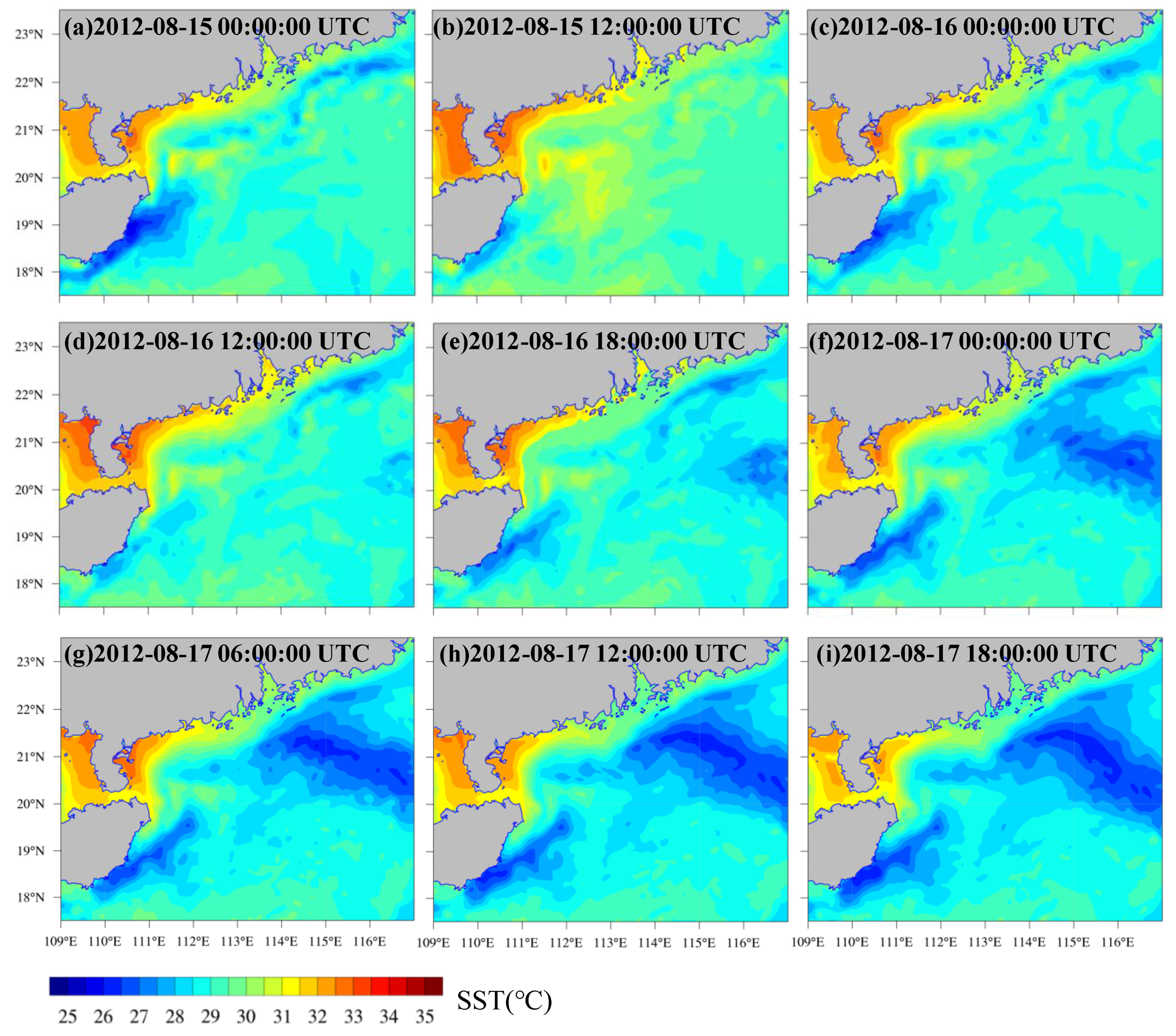
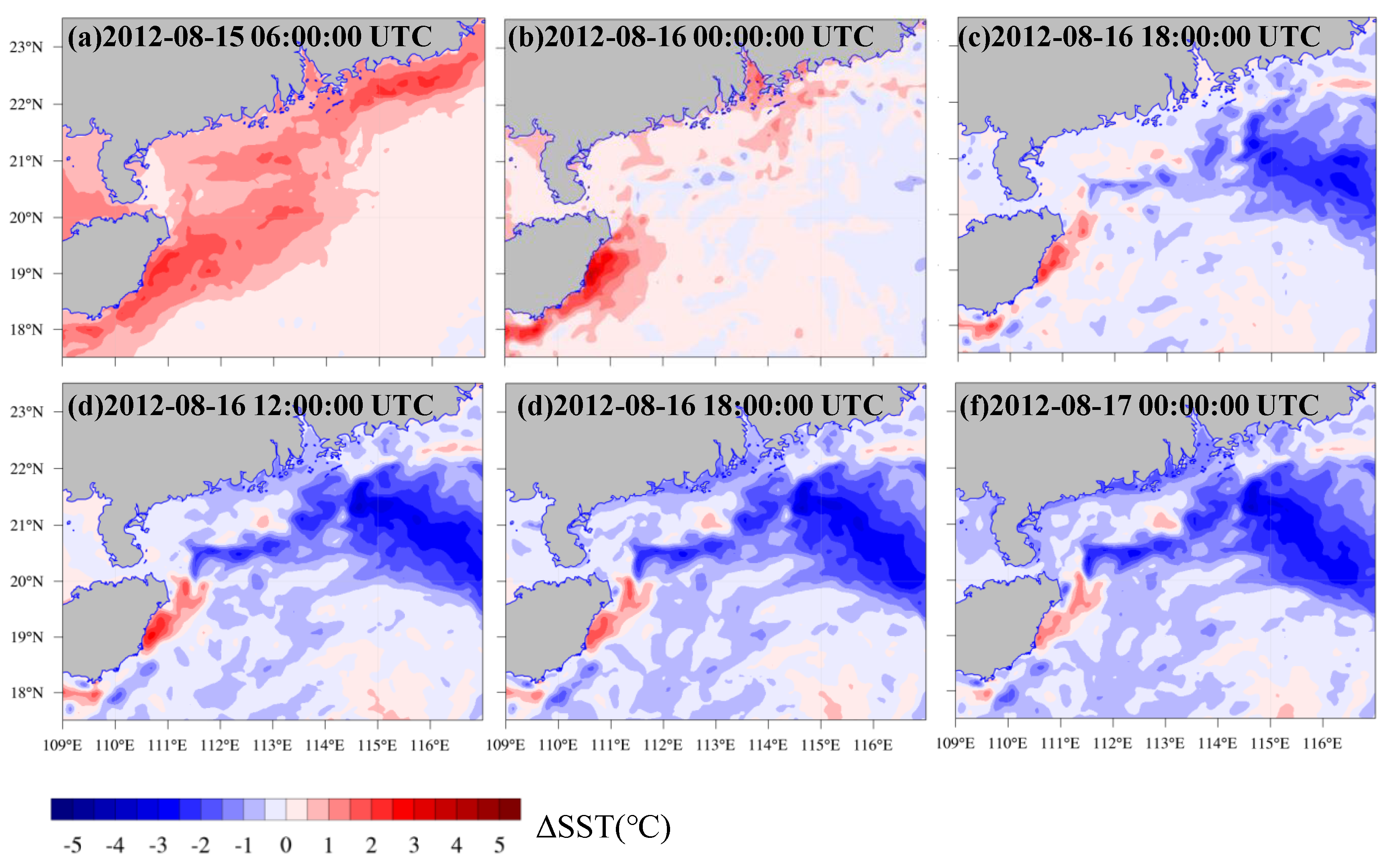
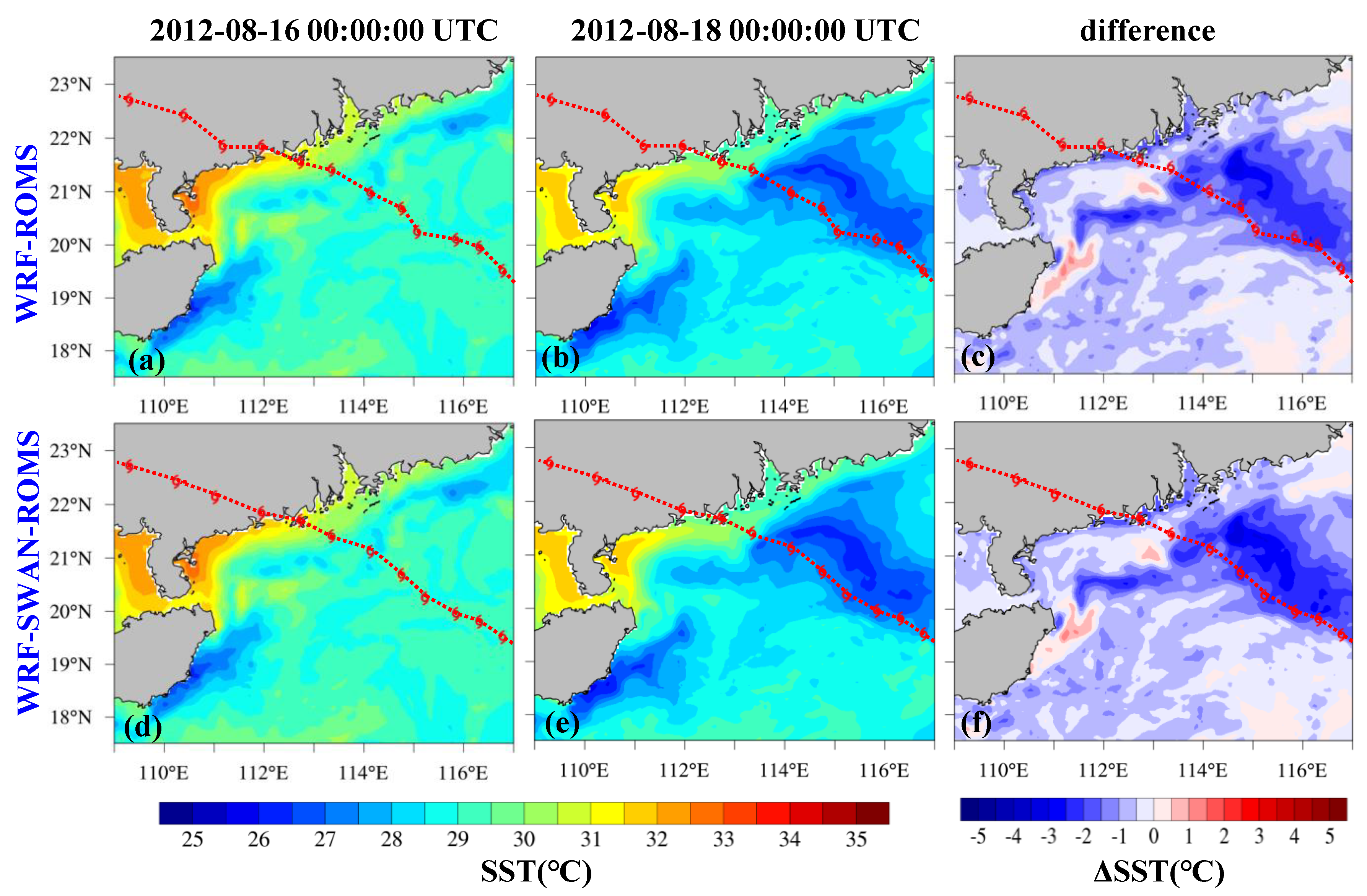
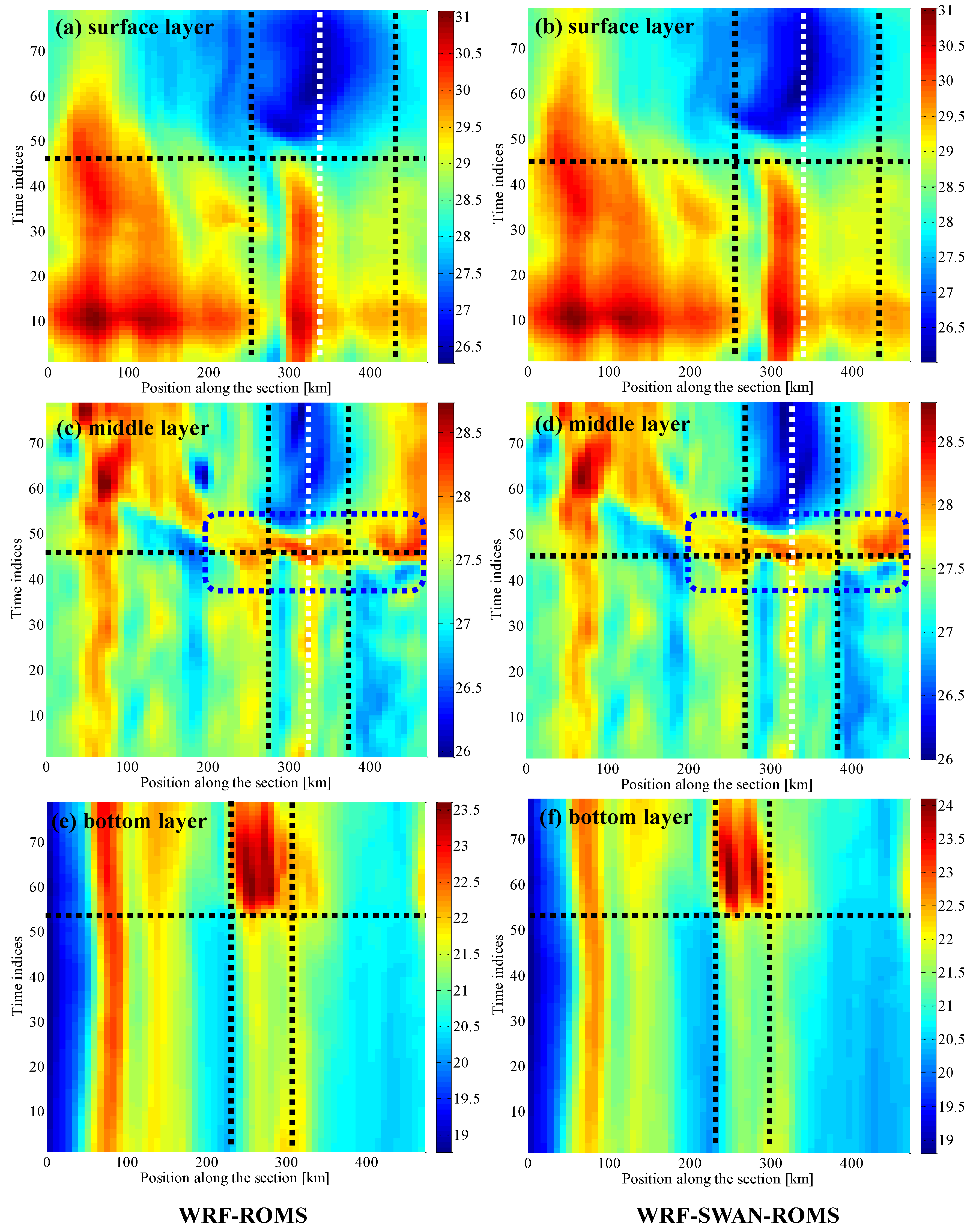
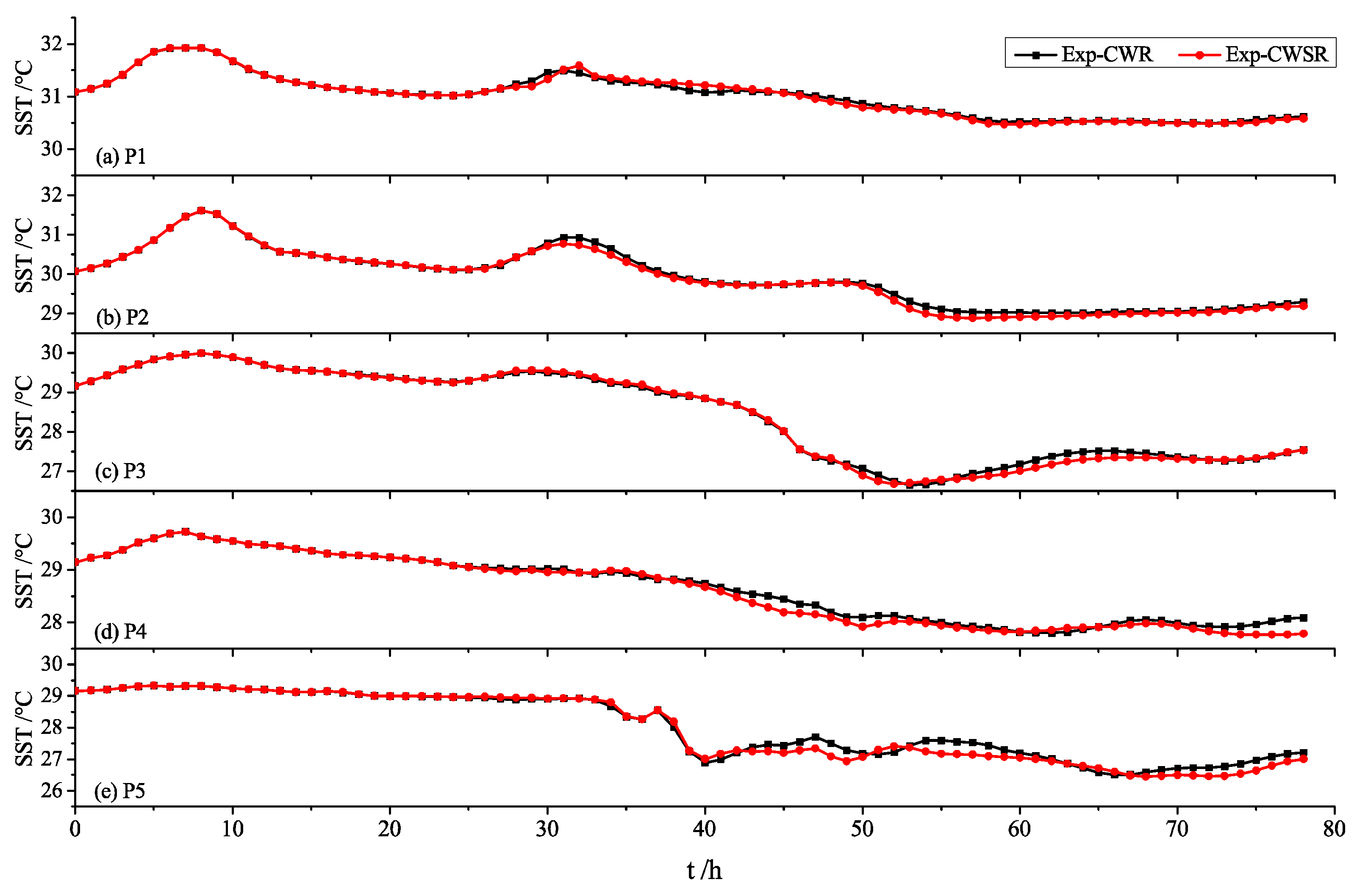
3.1. Sea Temperature

Under the influence of the typhoon, the sea surface temperature (SST) underwent a relatively obvious cooling process. The evolution process of the SST of the South China Sea, based on the fully coupled WRF-SWAN-ROMS model (Exp-CWSR) during the Typhoon Kai-tak, is shown in Figure 4. The change of the sea surface temperature (ΔSST) of the South China Sea before the impact of the typhoon based on the Exp-CWSR scheme and the reference time is 2012-08-15 00:00:00 UTC is shown in Figure 5.

As can be seen from Figure 5, in the early stage of the influence of the Typhoon Kai-tak, such as 2012-08-15 06:00:00 (UTC), that is, at 2012-08-15 14:00:00 (Beijing time), due to factors such as solar radiation, the sea receives external heat, causing an increase in SST: the temperature in the coastal ocean rose more than 3 °C. Beginning at 2012-08-15 12:00:00 (UTC), that is, at 2012-08-15 20:00:00 (Beijing time), the sea surface began to be cool and the SST decreased. At 2012-08-16 00:00:00 (UTC), due to the influence of the Typhoon Kai-tak, the sea surface temperature around the typhoon center dropped significantly, and the maximum ΔSST dropped more than 4 °C.

The sea surface temperature changes (ΔSST) under the influence of the typhoon also showed obvious spatial asymmetry. The SST drop on the right side of the typhoon track is significantly greater than the decrease in the SST on the left side. It can be seen from the figure that the SST on the right side of the typhoon track can reach above 4 °C, while the SST in the left side of the typhoon track is about 2 °C.

In order to further analyze the variation evolution of sea temperature under the influence of the typhoon, five characteristic locations were selected around the typhoon track as shown in Figure 6a, and the temperatures of sea surface, middle, and bottom and local air pressure were plotted as shown in Figure 6b–f. In the early stage of the influence by typhoon, due to the solar radiation and other factors, the heat exchange between air to sea and the sea surface temperature has a period rise and fall, especially in the coastal ocean zone (P1, P2), as shown by the red dashed box in Figure 6b,c.

Under the influence of the typhoon, the sea surface temperature in each characteristic location has dropped significantly. In the deep sea (P3, P4, and P5), the sea surface temperature drops by more than 3 °C; the sea surface temperature in the coastal ocean zone (P1 and P2) also drops by more than 1 °C. This is because the flow velocity at the bottom of the mixed layer is very large during the typhoon process, so that the cold water of the bottom layer is mixed with the upper ocean under the action of the pumping driven by typhoon, which leaded coastal ocean upwelling and the temperature of the mixed layer decreasing.

For the temperatures in the middle and bottom layer, the difference between the different locations is large as shown in Figure 6. For comparison, the correspondence between each characteristic position and the water depth contour is given in Figure 7. P1 and P2 are located outside the 10 m isobath, near the 20 m isobath; P3 is within the 100 m isobath, P4 is within the 200 m isobath; and P5 is within the 1000 m isobath.

The surface sea at the P5 position in the deep sea is cool about 4 °C caused by typhoon, but the middle and bottom waters are basically stable. At the P4 position, the strong Ekman pumping in the ocean caused by the strong vortex shear force driven by the typhoon, and the middle and bottom layers are both disturbed, so there were temperature amplitudes in the middle and bottom layers of the sea. The position of P3 is within the 100 m isobath, the middle layer has been completely disturbed by the influence of Ekman pumping, and the same change evolution as the sea surface temperature. However, the P1 and P2 in the coastal ocean zone, due to the shallow water, the water temperature of the entire section showed a similar trend. In terms of time, the decrease in sea temperature lags the moment when the extreme value of the air pressure occurs, that is, there is a temporal lag of the sea temperature response to the typhoon.

The comparison of SST and ΔSST based on the coupled WRF-ROMS model (Exp-CWR) and the fully coupled WRF-SWAN-ROMS model (Exp-CWSR) is shown in Figure 8. It can be seen from the figure that no matter which coupled schemes were applied, the spatial distribution of SST and ΔSST show an obvious spatial asymmetric characteristic, and the SST extreme position is located ~80 km to the right of the typhoon track.

Comparing the two different coupled schemes, it can be seen that after the impact of the typhoon, the ΔSST based on the Exp-CWSR scheme is slightly larger than the ΔSST based on the Exp-CWR scheme, and the change zone is relatively larger. It can be seen from the figure that in the fully coupled model, due to the addition of the wave model, the rough length ($z_0$, in Formula (2)) has increased, which caused the mixing effect of the surface water meaning that the bottom cool water is strengthened, and therefore, the sea surface temperature drop is more obvious.

In order to gain a deeper understanding of the variation characteristics of sea temperature under the influence of typhoon, section S1 intersecting the typhoon track near the 100 m isobath in the northern of the South China Sea had been selected as shown in Figure 7. The spatiotemporal distribution of simulated temperature in the surface layer, middle layer, and bottom layer on the S1 section in the Exp-CWR scheme and the Exp-CWSR scheme are plotted as shown in Figure 9.

From Figure 9a,b it can be found that the SST evolutions in the S1 section with time based on the two different schemes were basically consistent. The cooling moment was kept synchronous (black horizontal dashed line) and the cooling range (black vertical dashed line) and the SST extreme position (white vertical dashed line) were in good agreement.

From Figure 9c,d it can be found that there was a rise and fall process of the temperature in the middle layer based on both two coupled schemes (the blue dotted line in the figure). The strong Ekman pumping effect by typhoon caused the middle layer is mixed with the surface hot water, and then causing the sea temperature in the middle layer to rise. With the continuous action and strengthening of the typhoon, the cool water in the bottom layer produced an upwelling caused by the Ekman pumping, which reduced the temperature of the middle layer, while the temperature of the bottom layer continued to rise, as shown in Figure 9e,f. On the other hand, the sea surface temperature begins to decrease under the influence of the typhoon, so the temperature of the middle layer decreases under the action of mixing. Under the joint influence of these two factors, a process of first rising and then falling of the temperature in the middle layer had been generated.

Comparing Figure 9c,d, it can be seen that the difference of temperature in the middle layer simulated by the Exp-CWSR scheme is larger than that of the Exp-CWR scheme (white vertical dashed line), and the change range of temperature based on the Exp-CWSR scheme is larger (black vertical dashed line). This is because under the influence of the waves, the mixing effect of the ocean is strengthened, which is more conducive to the exchange of the cool water of the bottom layer with the hot water of the surface layer and the middle layer.

It can be seen from Figure 9e,f that the temperature of the cool water in the bottom layer continues to hot under the influence of typhoon. As discussed above, this is because the Ekman pumping has been continuously strengthened with the development of the typhoon, so that the bottom water continues to produce upwelling and mixing with the middle layer and the surface hot water, which caused the cool water in the bottom layer to be consistently hotter. In addition, comparing the range of extreme values of the temperature change in the bottom layer based on the two different schemes (black vertical dashed line), it can be found that from the surface layer to the bottom layer, the extreme values of the sea temperature of each layer gradually approach the center of the typhoon. This indicates that the spatial asymmetric distribution of surface water temperature is more obvious, and the asymmetry characteristic became to weaken with the increase of water depth.

The sea surface temperature evolution for each characteristic position (Figure 6a), obtained in the two different coupled schemes (Exp-CWR and Exp-CWSR), is shown in Figure 10. It can be seen from Figure 10 that the SST variation of each characteristic position based on the two different coupled schemes is basically the same. Compared with the two schemes, the SST obtained by the Exp-CWSR scheme has a larger amplitude and the response time to the typhoon is shorter, that is, the simulated SST in the fully coupled WRF-SWAN-ROMS model had be cooler, and the lag time is relatively shorter than the coupled WRF-ROMS model.

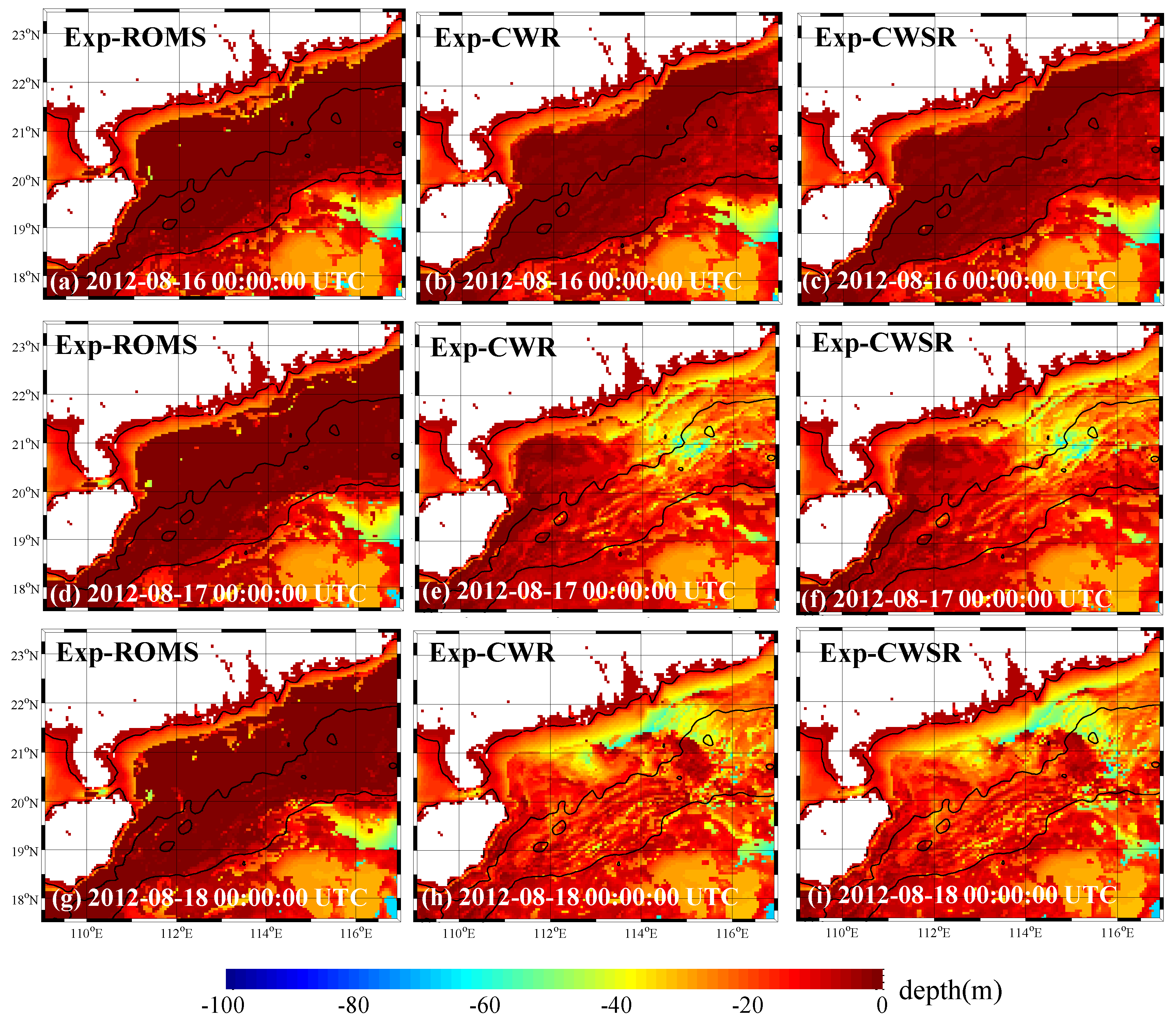
3.2. Mixed Layer Depth

The mixed layer depth (MLD), calculated at different times under the three different schemes (Exp-ROMS, Exp-CWR, and Exp-CWSR), is shown in Figure 11. The mixed layer depth is calculated by Lorbacher and Dommenget (2006) [36]. In the Exp-ROMS scheme, the mixed layer depth was calculated under the astronomical forcing condition during the influence of the Typhoon Kai-tak, and in the Exp-CWR and Exp-CWSR schemes, the mixed layer depth was calculated by different coupled schemes under the influence of the Typhoon Kai-tak. It can be seen from the figure that under the influence of the astronomical tide (Exp-ROMS), the spatial distribution of the mixed layer depth at different times is relatively stable (Figure 11a,d,g). Due to the influence of tidal and coastal currents in the coastal zone, the mixed layer depth can reach ~10 m. Outside of the 1000 m isobath, the mixed layer depth can reach ~60 m in the deep sea. From the 30 m isobath to the 1000 m isobath, the mixed layer depth is approximately 10 m.

In the Exp-CWR and Exp-CWSR schemes, the spatial distribution of the mixed layer depth under the influence of Typhoon Kai-tak is significantly different from that of the Exp-ROMS scheme. In the early stage of the influence of the storm surge, at 2012-08-16 00:00:00 UTC, the mixed layer depth in the South China Sea was similar to that under the influence of the astronomical tide. It can be seen from the figure that at 2012-08-17 00:00:00 UTC, the mixed layer depth under the influence of storm surge caused by Typhoon Kai-tak based on the Exp-CWR and Exp-CWSR schemes is significantly greater than the mixed layer depth under the influence of the astronomical tide.

Comparing the distribution of mixed layer depth based on the Exp-CWR and Exp-CWSR schemes, we find that the spatial distribution of mixed layer depth is similar. Under the influence of the typhoon, the mixed layer depth in the entire calculation domain had increased. Due to the strong vortex shear force caused by the typhoon, strong Ekman pumping is induced, so the mixed layer depth near the typhoon track is large. In the coastal ocean zone from the 30 m isobath to the 100 m isobath, the mixed layer depth can reach more than 60 m, which means that almost all the ocean in the entire section was mixed by the typhoon. Comparing the two different coupled schemes, it can be found that the mixed layer depth calculated on the Exp-CWSR scheme is slightly larger than that of the Exp-CWR scheme, which further confirms that the wave action leads to the intensification of vertical mixing.

4. Discussions

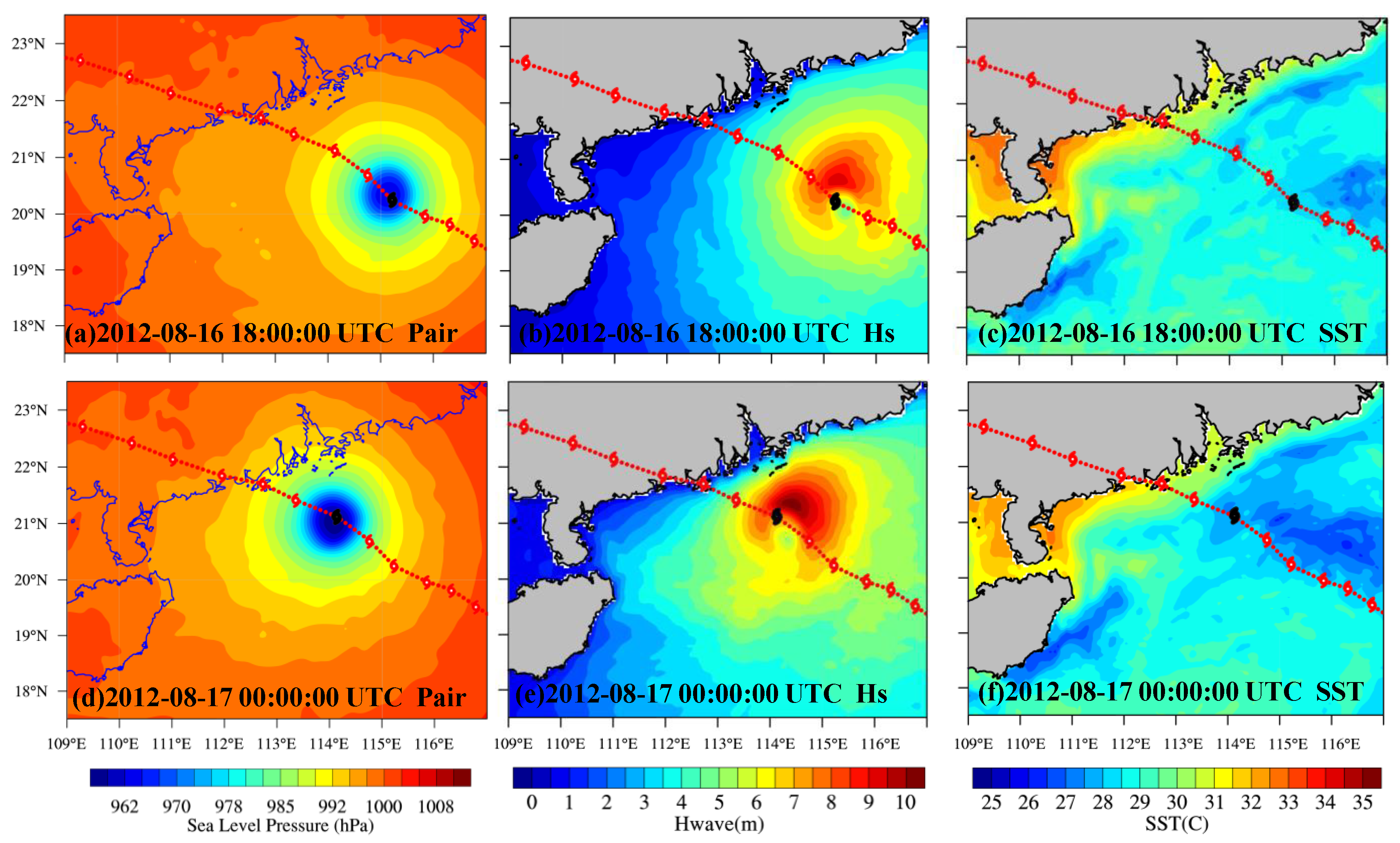
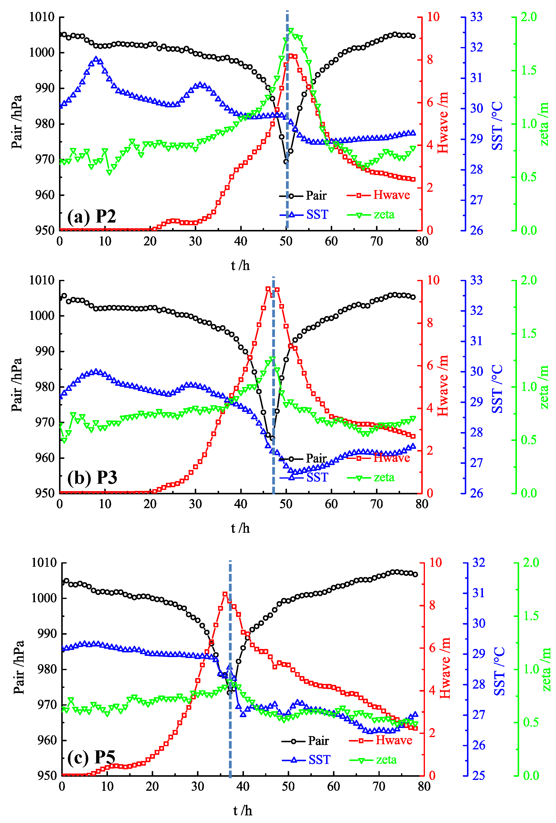
4.1. Correspondence Relationships between the Atmospheric, Waves and Oceanic Factors

Atmospheric, waves, and oceanic results in different coupled schemes are described and analyzed in the Section 3. The mutual coupled relationships between the atmospheric, waves, and oceanic factors is discussed in this section. The spatial distribution of sea level pressure, wave height, and sea surface temperature at 2012-08-16 18:00:00 UTC and 2012-08-17 00:00:00 UTC based on the Exp-CWSR scheme is shown in Figure 12. In the Figure 12, the air pressure is used to represent the atmospheric results, the wave height represents the wave results, and the sea surface temperature represents the oceanic results. The red dashed line in the figure is the typhoon track, and the black circle is marked as the center of the typhoon at that time.

It can be seen from the Figure 12 that the temporal and spatial distribution characteristics of the atmospheric, waves, and oceanic results are different. In temporal view, the response of the waves to the typhoon is relatively rapid, and the extreme value of the wave height is slightly later than the extreme value of the sea level pressure; while the response of the sea surface temperature to the typhoon is relatively slow, with obvious hysteresis characteristics of temporal lag.

From the perspective of spatial distribution, the distribution of sea level pressure along the typhoon track is relatively symmetrical. From the intensity of the contour line, it can be found that the pressure gradient on the right side of the typhoon track is larger, and from the previous analysis, we knew that the wind speed on the right side of the typhoon track is significantly larger than the left side. Therefore, the atmospheric results under the influence of typhoon are basically symmetrically distributed but have the reinforcement characteristics in the right side of the spatial distribution.

For wave height, its spatial distribution has obvious asymmetric distribution characteristics, and the wave height on the right side of the typhoon track is significantly larger than the left side. The spatial distribution of sea surface temperature has similar characteristics, the SST was decreased under the influence of typhoon, and the ΔSST on the right side of the typhoon track is greater than the ΔSST on the left side. The temporal and spatial distribution characteristics of the atmospheric, waves, and oceanic results are discussed below, respectively.

4.2. Temporal Distribution Characteristics

The evolution of sea level pressure, wave height, and sea surface temperature and wave level at the three characteristic positions (P2, P3, and P5 in Figure 8) under the influence of Typhoon Kai-tak, based on the fully coupled WRF-SWAN-ROMS model (Exp-CWSR), is shown in Figure 13.

It can be seen from Figure 13 that the air pressure, wave height, and water level had good correspondence and synchronization in time. The response of SST to typhoon is obviously hysteresis of temporal lag, indicating that it took an amount of time to deepen the strong mixing of the upper ocean and the mixed layer depth caused by typhoon. It can be seen from Figure 13c that in the deep sea zone (P5), the sea surface temperature is still decreasing two days after the typhoon landed.

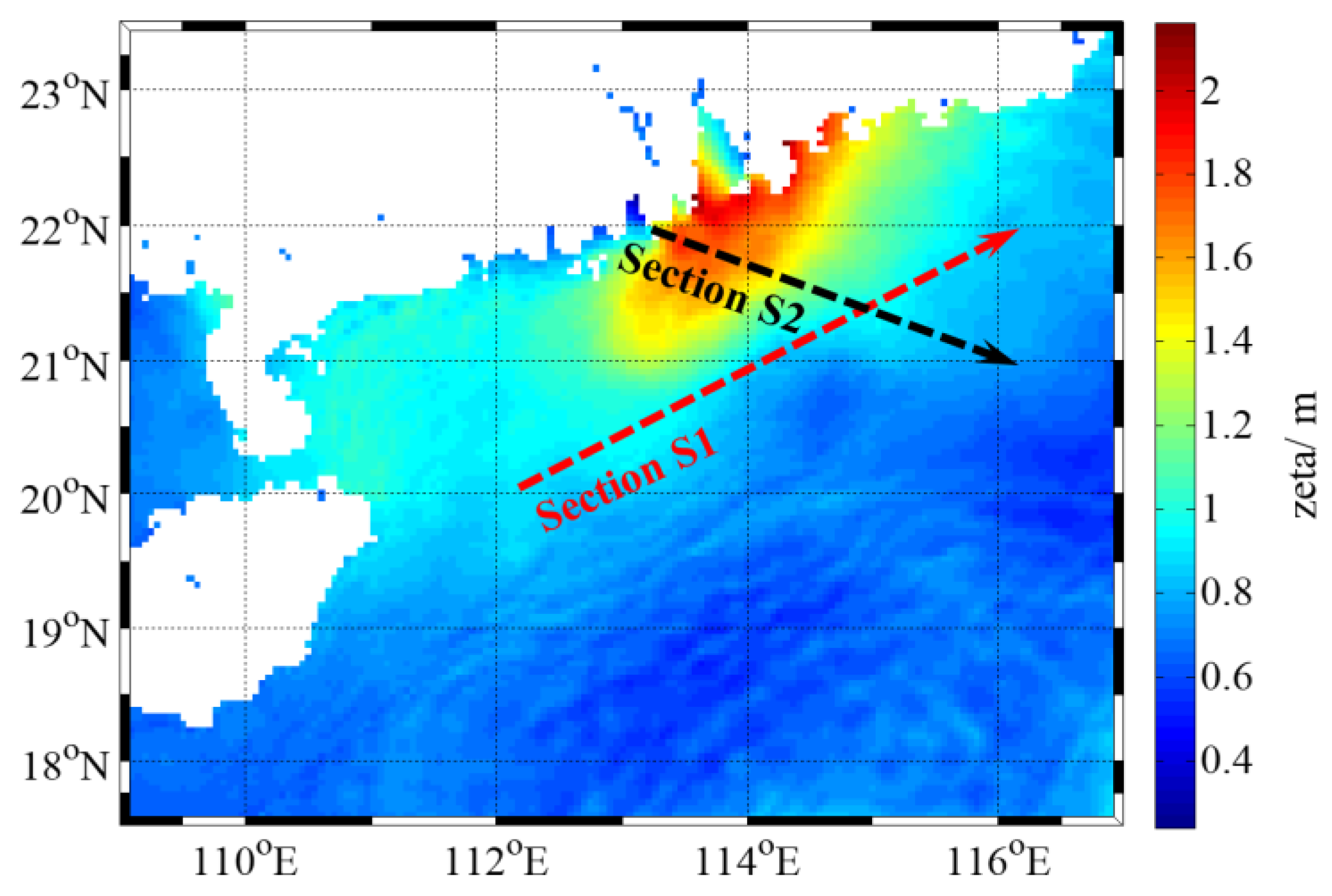
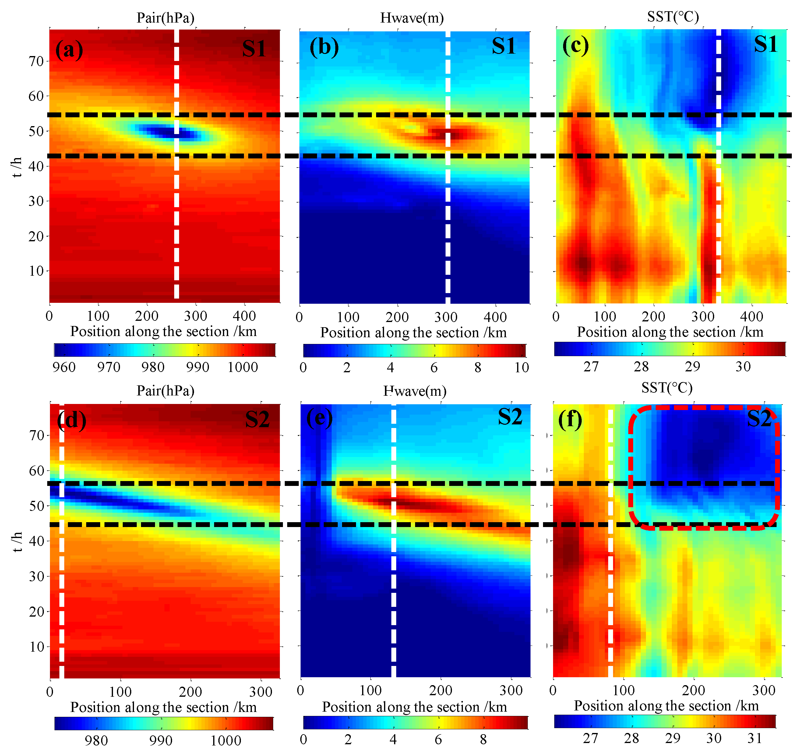
4.3. Spatial Asymmetry Distribution Characteristics

In order to discuss the spatial asymmetry distribution characteristics of waves and oceanic results, two characteristic sections are selected in the northern of the South China Sea as shown in Figure 14. The temporal and spatial distribution of sea level pressure, wave height, and sea surface temperature on these two sections under the influence of Typhoon Kai-tak are drawn, as shown in Figure 15.

It can be seen from Figure 15b that the wave height distribution on the S1 section under the influence of the Typhoon Kai-tak has obvious asymmetric spatial distribution characteristics: the wave height on the right side is high and the wave height on the left side is small. The reasons for the asymmetric distribution characteristics of typhoon waves include the following two points.

On the one hand, because the typhoon intensity on the right side of the typhoon track is stronger than the left side because of the Coriolis force, the wave height on the right side of the typhoon track is larger than the left side under the same conditions. On the other hand, in the right front of the typhoon center, the direction of wave propagation is consistent with the direction of typhoon movement. The wave in front of the typhoon center can continuously obtain energy from the typhoon wind field during the propagation process, and the wind fetch in this zone is large. As a result, the wave height increased because the energy of the waves in the zone continued to increase. The wave located at the left rear of the typhoon center cannot continuously obtain energy from the typhoon due to the direction of wave propagation is opposite to the direction of typhoon movement, that is, the wind fetch is smaller. Therefore, the wave height at the right front of the typhoon center is significantly larger than the left rear.

5. Conclusions

In this study, the fully coupled Atmosphere–Wave–Ocean model of the South China Sea based on the COAWST model system is established and applied to the simulation of the storm surge in the South China Sea under the influence of Typhoon Kai-tak. The temporal and spatial distribution of sea temperature and mixed layer depth had been simulated and discussed. The simulation results of different four coupled schemes have been compared with the each other.

The spatial and temporal distribution of temperature field and vertical mixing layer depth under the influence of Typhoon Kai-tak had been calculated based on the fully coupled WRF-SWAN-ROMS model. The simulation results show that the fully coupled WRF-SWAN-ROMS model shows that the typhoon passes through the sea with obvious cooling. In the cold eddy region, the cooling of the sea surface temperature at 4 to 5 °C occurs, and the cooling zone is concentrated on the right side of the track. The change of sea surface temperature lags behind the change of sea surface height more than 12 h. The decrease of SST on the left side of the track was relatively small, ranging from 1.5 to 2.5 °C. The disturbance of typhoon causes the subsurface water to surge to the surface, changes the temperature distribution of the surface, and causes the mixing layer to deepen ~40–60 m. The simulation results reveal the temporal and spatial distribution of sea temperature and mixed layer depth. The sea surface temperature field has an asymmetrical distribution in space and has lag in time. The heat exchange at the air–sea interface is very strong under the influence of typhoon, and the latent heat generated by water vapor evaporation plays a dominant role in the heat exchange at the air–sea interface, which shows that the heat carried by the vaporization of the sea surface is one of the important factors contributing to the decrease of sea temperature under the influence of the typhoon.

Due to the limitation of field observation data, only a few numerical simulation results are validated in this paper, and the reliability of the model may be questioned. We hope that in future research, more actual typhoon examples and observation data can be used to test the reliability of the model.

References

1. Song, D.; Guo, L.; Duan, Z.; Xiang, L. Impact of Major Typhoons in 2016 on Sea Surface Features in the Northwestern Pacific. Water 2018, 10, 1326. [Google Scholar] [CrossRef]
2. Chia, H.H.; Ropelewski, C.F. The interannual variability in the genesis location of tropical cyclones in the northwest Pacific. J. Clim. 2002, 15, 2934–2944. [Google Scholar] [CrossRef]
3. Wang, G.; Su, J.; Ding, Y. Tropical cyclone genesis over the South China Sea. J. Mar. Syst. 2007, 68, 318–326. [Google Scholar] [CrossRef]
4. Yasuda, T.; Nakajo, S.; Kim, S.Y. Evaluation of future storm surge risk in East Asia based on state-of-the-art climate change projection. Coast. Eng. 2014, 83, 65–71. [Google Scholar] [CrossRef]
5. Sun, J.; Wang, G.; Zuo, J. Role of surface warming in the northward shift of tropical cyclone tracks over the South China Sea in November. Acta Oceanol. Sin. 2017, 36, 67–72. [Google Scholar] [CrossRef]
6. Emanuel, K. Increasing destructiveness of tropical cyclones over the past 30 years. Nature 2005, 436, 686–688. [Google Scholar] [CrossRef] [PubMed]
7. Webster, P.J.; Holland, G.J.; Curry, J.A. Changes in tropical cyclone number, duration, and intensity in a warming environment. Science 2005, 309, 1844–1846. [Google Scholar] [CrossRef] [PubMed]
8. Lee, T.L. Neural network prediction of a storm surge. Ocean Eng. 2006, 33, 483–494. [Google Scholar] [CrossRef]
9. Almar, R.; Marchesiello, P.; Almeida, L.P.; Thuan, D.H.; Tanaka, H.; Viet, N.T. Shoreline Response to a Sequence of Typhoon and Monsoon Events. Water 2017, 9, 364. [Google Scholar] [CrossRef]
10. Mei, X.; Dai, Z.; Darby, S.E. Modulation of extreme flood levels by impoundment significantly offset by floodplain loss downstream of the Three Gorges Dam. Geophys. Res. Lett. 2018, 45, 3147–3155. [Google Scholar] [CrossRef]
11. Wu, Z.; Jiang, C.; Deng, B.; Chen, J.; Li, L. Evaluation of numerical wave model for typhoon wave simulation in South China Sea. Water Sci. Eng. 2018, 11, 229–235. [Google Scholar] [CrossRef]
12. Wu, G.; Li, H.; Liang, B. Subgrid modeling of salt marsh hydrodynamics with effects of vegetation and vegetation zonation. Earth Surf. Process. Landf. 2017, 42, 1755–1768. [Google Scholar] [CrossRef]
13. Wu, G.; Shi, F.; Kirby, J.T. Modeling wave effects on storm surge and coastal inundation. Coast. Eng. 2018, 140, 371–382. [Google Scholar] [CrossRef]
14. Yin, X.; Wang, Z.; Liu, Y. Ocean response to Typhoon Ketsana traveling over the northwest Pacific and a numerical model approach. Geophys. Res. Lett. 2007, 34, 21606. [Google Scholar] [CrossRef]
15. Chen, W.-B.; Lin, L.-Y.; Jang, J.-H.; Chang, C.-H. Simulation of Typhoon-Induced Storm Tides and Wind Waves for the Northeastern Coast of Taiwan Using a Tide–Surge–Wave Coupled Model. Water 2017, 9, 549. [Google Scholar] [CrossRef]
16. Potter, H.; Drennan, W.M.; Graber, H.C. Upper ocean cooling and air-sea fluxes under typhoons: A case study. J. Geophys. Res. Oceans 2017, 122, 7237–7252. [Google Scholar] [CrossRef]
17. Li, Z.L.; Wen, P. Comparison between the response of the Northwest Pacific Ocean and the South China Sea to Typhoon Megi (2010). Adv. Atmos. Sci. 2017, 34, 79–87. [Google Scholar] [CrossRef]
18. Chen, Y.; Yu, X. Enhancement of wind stress evaluation method under storm conditions. Clim. Dyn. 2016, 47, 3833–3843. [Google Scholar] [CrossRef]
19. Chen, Y.; Yu, X. Sensitivity of storm wave modeling to wind stress evaluation methods. J. Adv. Model. Earth Syst. 2017, 9, 893–907. [Google Scholar] [CrossRef]
20. Fan, Y.; Ginis, I.; Hara, T. The effect of wind–wave–current interaction on air–sea momentum fluxes and ocean response in tropical cyclones. J. Phys. Oceanogr. 2009, 39, 1019–1034. [Google Scholar] [CrossRef]
21. Gronholz, A.; Gräwe, U.; Paul, A. Investigating the effects of a summer storm on the North Sea stratification using a regional coupled ocean-atmosphere model. Ocean Dyn. 2017, 67, 1–25. [Google Scholar] [CrossRef]
22. Mattocks, C.; Forbes, C. A real-time, event-triggered storm surge forecasting system for the state of North Carolina. Ocean Model. 2008, 25, 95–119. [Google Scholar] [CrossRef]
23. Xu, S.; Huang, W.; Zhang, G. Integrating Monte Carlo and hydrodynamic models for estimating extreme water levels by storm surge in Colombo, Sri Lanka. Nat. Hazards 2014, 71, 703–721. [Google Scholar] [CrossRef]
24. Zhang, K.; Li, Y.; Liu, H. Transition of the coastal and estuarine storm tide model to an operational storm surge forecast model: A case study of the Florida coast. Weather Forecast. 2013, 28, 1019–1037. [Google Scholar] [CrossRef]
25. Black, P.G.; D’Asaro, E.A.; Sanford, T.B. Air-sea exchange in hurricanes: Synthesis of observations from the coupled boundary layer air–sea transfer experiment. Bull. Am. Meteorol. Soc. 2007, 88, 357–374. [Google Scholar] [CrossRef]
26. Chen, Y.; Zhang, F.; Green, B.W. Impacts of Ocean Cooling and Reduced Wind Drag on Hurricane Katrina (2005) Based on Numerical Simulations. Mon. Weather Rev. 2018, 146, 287–306. [Google Scholar] [CrossRef]
27. Liu, B.; Liu, H.; Xie, L. A Coupled Atmosphere-Wave-Ocean Modeling System: Simulation of the Intensity of an Idealized Tropical Cyclone. Mon. Weather Rev. 2010, 139, 132–152. [Google Scholar] [CrossRef]
28. Mori, N.; Kato, M.; Kim, S. Local amplification of storm surge by Super Typhoon Haiyan in Leyte Gulf. Geophys. Res. Lett. 2014, 41, 5106–5113. [Google Scholar] [CrossRef] [Green Version]
29. Takagi, H.; Esteban, M.; Shibayama, T. Track analysis, simulation, and field survey of the 2013 Typhoon Haiyan storm surge. J. Flood Risk Manag. 2017, 10, 42–52. [Google Scholar] [CrossRef]
30. Yin, K.; Xu, S.; Huang, W. Effects of sea level rise and typhoon intensity on storm surge and waves in Pearl River Estuary. Ocean Eng. 2017, 136, 80–93. [Google Scholar] [CrossRef]
31. Wang, J.; Yi, S.; Li, M. Effects of sea level rise, land subsidence, bathymetric change and typhoon tracks on storm flooding in the coastal areas of Shanghai. Sci. Total Environ. 2018, 621, 228–234. [Google Scholar] [CrossRef] [PubMed]
32. Warner, J.C.; Sherwood, C.R.; Signell, R.P. Development of a three-dimensional, regional, coupled wave, current, and sediment-transport model. Comput. Geosci. 2008, 34, 1284–1306. [Google Scholar] [CrossRef]
33. Warner, J.C.; Armstrong, B.; He, R. Development of a Coupled Ocean–Atmosphere–Wave–Sediment Transport (COAWST) Modeling System. Ocean Model. 2010, 35, 230–244. [Google Scholar] [CrossRef] [Green Version]
34. Charnock, H. Wind stress on a water surface. Q. J. R. Meteorol. Soc. 1955, 81, 639–640. [Google Scholar] [CrossRef]
35. Taylor, P.K.; Yelland, M.J. The dependence of sea surface roughness on the height and steepness of the waves. J. Phys. Oceanogr. 2001, 31, 572–590. [Google Scholar] [CrossRef]
36. Lorbacher, K.; Dommenget, D.; Niiler, P.P. Ocean mixed layer depth: A subsurface proxy of ocean-atmosphere variability. J. Geophys. Res. Oceans 2006, 111, 520–522. [Google Scholar] [CrossRef]
Figure 1. The simulation domain of the coupled WRF-SWAN-ROMS model in the South China Sea.
Water 11 00140 g001
Figure 2. The topography of the South China Sea (unit: m).
Water 11 00140 g002
Figure 3. The track and satellite image of typhoon Kai-tak and the buoy station and in-site station. (a) typhoon track; (b) satellite image.
Water 11 00140 g003
Figure 4. The spatial distribution of sea surface temperature (SST) in the northern area of the South China Sea under the influence of Typhoon Kai-tak, based on the Exp-CWSR scheme.
Water 11 00140 g004
Figure 5. The spatial distribution of change in sea surface temperature (ΔSST) in the northern area of the South China Sea under the influence of Typhoon Kai-tak, based on the Exp-CWSR scheme (reference time 2012-08-15 00:00:00 UTC).
Water 11 00140 g005
Figure 6. The variation of the temperature of the sea surface, middle, and bottom and air pressure at five characteristic locations during Typhoon Kai-tak (start at 2012-08-15 00:00:00 UTC).
Water 11 00140 g006
Figure 7. Schematic diagram of relative position of each characteristic position and isobath.
Water 11 00140 g007
Figure 8. The comparison of SST and ΔSST in two different schemes (unit: °C). (a,b) is the SST at 2012-08-16 00:00:00 UTC and 2012-08-18 00:00:00 UTC based on the Exp-CWR. (d,e) is the SST at 2012-08-16 00:00:00 UTC and 2012-08-18 00:00:00 UTC based on the Exp-CWSR. (c,f) is the ΔSST based on the two different schemes.
Water 11 00140 g008
Figure 9. Temporal and spatial distribution of sea temperature in the three different layers on the S1 section during the Typhoon Kai-tak based on the two different schemes (start at 2012-08-15 00:00:00 UTC).
Water 11 00140 g009
Figure 10. The evolution of SST in five characteristic positions over time in the two different coupled schemes.
Water 11 00140 g010
Figure 11. The spatial distribution of mixed layer depth (MLD) in the northern area of the South China Sea under the influence of Typhoon Kai-tak, based on the three different schemes.
Water 11 00140 g011
Figure 12. The spatial distribution of sea level pressure, wave height, and sea surface temperature in the northern area of the South China Sea under the influence of Typhoon Kai-tak, based on the fully coupled WRF-SWAN-ROMS model (Exp-CWSR).
Water 11 00140 g012
Figure 13. The evolution of sea level pressure, wave height, sea surface temperature, and wave level at three characteristic positions during Typhoon Kai-tak based on the Exp-CWSR scheme (start at 2012-08-15 00:00:00 UTC).
Water 11 00140 g013
Figure 14. Schematic diagram of the location of the two characteristic sections.
Water 11 00140 g014
Figure 15. The temporal and spatial distribution of sea level pressure, wave height, and sea surface temperature in the S1 and S2 under the influence of Typhoon Kai-tak based on the Exp-CWSR (start at 2012-08-15 00:00:00 UTC).
Water 11 00140 g015