Calibration of SWAT and Two Data-Driven Models for a Data-Scarce Mountainous Headwater in Semi-Arid Konya Closed Basin

Abstract

Hydrologic models are important tools for the successful management of water resources. In this study, a semi-distributed soil and water assessment tool (SWAT) model is used to simulate streamflow at the headwater of Çarşamba River, located at the Konya Closed Basin, Turkey. For that, first a sequential uncertainty fitting-2 (SUFI-2) algorithm is employed to calibrate the SWAT model. The SWAT model results are also compared with the results of the radial-based neural network (RBNN) and support vector machines (SVM). The SWAT model performed well at the calibration stage i.e., determination coefficient (R²) = 0.787 and Nash–Sutcliffe efficiency coefficient (NSE) = 0.779, and relatively lower values at the validation stage i.e., R² = 0.508 and NSE = 0.502. Besides, the data-driven models were more successful than the SWAT model. Obviously, the physically-based SWAT model offers significant advantages such as performing a spatial analysis of the results, creating a streamflow model taking into account the environmental impacts. Also, we show that SWAT offers the ability to produce consistent solutions under varying scenarios whereas it requires a large number of inputs as compared to the data-driven models.

1. Introduction

The studies of hydrological modelling play a crucial role in planning water resources, projecting hydraulic structures, and evaluating environmental impacts [1,2,3,4]. The estimation of accurate streamflow is required for the estimation of floods, development of agricultural strategies, and planning of hydraulic structures. [5,6,7]. Although streamflow estimation studies are required for hydrological assessment, there are some difficulties in implementation. Conducting a comparative study with different estimation methods ensures successful interpretation of the outputs and produced more reliable results. Physically based models (soil and water assessment tool (SWAT), topography based hydrological model (TOPMODEL), European hydrologic system (SHE), etc.) and artificial intelligence (AI) models are frequently used for modelling hydrological problems.

Hydrological models can be classified as physical, mathematical (including distributed physically based models and lumped conceptual) and empirical models. Physically based models allow the mathematical solution by transferring the nature events to a computer simulation program. These models are suitable tools for analyzing the process and the factors affecting the process, as well as the results in the modeling of hydrological events. A lot of data is needed to transfer the hydrological process to the computer simulation program in physically based models. Data-driven models such as AI, computational intelligence (CI), soft computing (SC), machine learning (ML), and data mining (DM) are based on analyzing system-related data and linking among input and output variables, without explicit knowledge of the physical behavior of the system [8]. In addition, adequate data should be provided for the training process in data-driven models. SWAT, a physically-based model frequently used by different disciplines, evaluates the watershed from a wider perspective [9,10,11,12,13,14]. The SWAT model is widely used in the simulation of the quality and quantity of surface and groundwater, in estimating the environmental impacts of different land use/land management practices and climate change, in calculating loads from pollutants, in evaluating best management practices, and in the simulation of various hydrological processes (runoff, infiltration, evapotranspiration, lateral flow, tile drainage, return flow, sediment etc) [15]. SWAT employs two different methods, the soil conservation services-curve number (SCS-CN) and the Green Ampt-MeinLarsen, for streamflow estimation [16,17,18,19]. Concurrent use of a digital elevation model (DEM), land use/land cover (LULC), and soil map alongside meteorological inputs also enables spatial analysis of the outputs produced by the model. As it includes physical inputs, the SWAT model yields successful results also in ungauged catchments [20,21].

AI models such as support vector machines (SVM), artificial neural networks (ANN) and adaptive network-based fuzzy inference system (ANFIS) are widely used in estimating hydrological and meteorological phenomena. Tongal [22] used a chaotic approach (k-nearest neighbor-kNN) and neural networks (feed-forward neural networks, FFNN) the non-linear estimation of the streamflow of Yamula station in Kızılırmak Basin and found that the kNN model was more successful than the FFNN model for streamflow estimation. Buyukyildiz et al. [23] used five different methods, including support vector regression (SVR), artificial neural networks based on particle swarm optimization (PSO-ANN), radial-based neural networks (RBNN), multi-layer artificial neural networks (MLP), and ANFIS to estimate change of the monthly water level in Lake Beyşehir and found that the ε-SVR model (R² = 0.9988) was more successful than the other models. Temizyurek and Dadaser-Celik [24] modeled the water temperature directly affecting biological and chemical processes within the stream using artificial neural networks. The best results were obtained by sigmoid activation function and the scaled conjugate gradient algorithm. Radzi et al. [25] used ANN, ANFIS and SVM, to estimate streamflow. The SVM method showed better results than ANFIS and ANN in estimating the daily mean fluctuation of the stream’s flow. Zhu et al. [26] evaluated the performances of the SVM coupled with discrete wavelet transform (DWT) and empirical mode decomposition (EMD) for streamflow estimation of Jinsha River in China. Hamaamin et al. [27] used the SWAT to predict streamflow in the Saginaw River Watershed of Michigan. The results were also compared with Bayesian regression and ANFIS.

The implementation of models with different approaches to the same problem is performed at the stage of testing the accuracy of the applications of many water resources. Besides, it allows exploring both advantages and disadvantages of the models. Demirel et al. [28] compared the daily streamflow estimations for Pracana watershed by means of SWAT and ANN models, and determined that the ANN model yielded the highest accuracy ratio. Jajarmizadeh et al. [29] performed monthly streamflow estimations for southern Iran using the SWAT and SVM models. Although high accuracy levels were achieved with both models, the SVM model was found to be more successful in estimation study. Noori and Kalin [30] applied SWAT and ANN models in order to perform streamflow estimations at 29 watersheds located around Atlanta during hot and cold seasons. At the end of the study, higher accuracy was attained in hot seasons than in cold seasons.

To the best of our knowledge, there is no study regarding streamflow estimation by using the SWAT model on the headwater of a watershed which has data scarcity and is in a mountainous region in Turkey. The main purpose of this study is to compare the physically based SWAT model and the non-process based AI models (RBNN and SVR) for streamflow estimation. A comparison of factors that affect the success of the model was conducted and it was determined that which model could be used for the solution of the problem. This study will provide a basis for the use of local and public administrations in improving a successful watershed management strategy in the Konya Closed Basin which has an arid and semi-arid climate.

2. Materials and Methods

2.1. Study Area

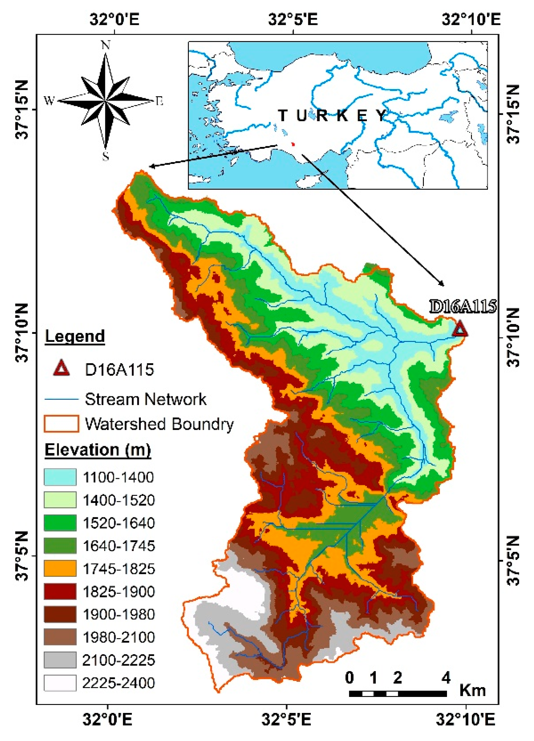
To compare the accuracy of SWAT and ANN/SVR models, the headwater of Çarşamba River Basin (in Turkey) was selected as a case study. Figure 1 shows the location map and the DEM map of the watershed. The studied area located in Konya Closed Basin in Turkey (Figure 1) is the headwater of the Çarşamba River Basin, which has a drainage area of 153.87 km² and has an elevation range from 1100 to 2400 m. This area is located between 37°14′ to 37°01′ north latitude and 31°58′ to 32°11′ east longitude. Mean annual precipitation, mean maximum temperature and mean minimum temperature is 785 mm, 17.5 °C and 6.1 °C, respectively. In the study area, forests, rocks, and annual plants correspond to 8.5%, 41% and 50.5% of the watershed, respectively. The D16A115 is the first streamflow gauging station in the headwater of the Çarşamba River. According to long-term annual measurements, the highest flow was observed in April (6.329 m³/s) while the lowest flow was observed in September (0.385 m³/s). Furthermore, long-term annual mean streamflow was observed to be 2.24 m³/s. The highest flow rate instantly observed at this station was measured as 60.8 m³/s during the flood on 15 December 2010.

2.2. Soil and Water Assessment Tool (SWAT)

SWAT developed by Arnold et al. [16] is a physically-based semi-distributed model. SWAT is an effective tool for assessing changes in hydrological processes (streamflow, sediment, etc.), erosion, and determination of agricultural origin pollutants in river basins, growth of vegetation, water quality in large river basins and effects of climate change on water resources management.

The SWAT model provides a simulation of a high-level of spatial detail by dividing the basin into a large number of sub-basins. The large-scale spatial heterogeneity of the study area is represented by the division of the basin into the sub-basins. Each sub-basin is separated into a series of hydrological response units (HRUs), which are unique soil-land use combinations. The fact that it divides a watershed into sub-basins ensures heterogeneity. The successful representation of the basin by the model is related to the provision of heterogeneity of the basin. The HRUs, defined as the smallest spatial units of the model representing LULC, soil types, and slopes within a subbasin based upon a user-defined threshold. The water flow is modeled by the analysis of HRUs.

SWAT is a physically-based model that simulates the hydrological cycle based on water balance controlled by climate inputs such as daily precipitation, maximum and minimum air temperature. In the SWAT model, water balance is conceptualized using Equation (1) [31].

$$S{W}_t=S{W}_0+{\displaystyle \sum }_{i=1}^t\left(R_{day}-Q_{surf}-E_a-W_{seep}-Q_{gw}\right)$$

(1)

where:

• SW_t: Final soil water content (mm);
• SW₀: Initial soil water content (mm);
• R_day: Amount of precipitation on day i (mm);
• Q_surf: Amount of surface runoff on day i (mm);
• E_a: Amount of evapotranspiration on day i (mm);
• W_seep: Amount of percolation and bypass flow exiting the soil profile bottom on day i (mm);
• Q_gw: Groundwater return flow on day i (mm).

The SCS-CN is a method used by SWAT for calculating surface runoff [32]. In SWAT, potential evapotranspiration (PET) is calculated by using three different methods including the Penman–Monteith, Hargreaves and Priestley–Taylor. Groundwater flow is important in basins with high hydraulic conductivity and a kinematic storage model based on continuity and water budget equations is used for modeling groundwater [31]. Model equations and more detailed descriptions (model use, calibration and validation etc) are available in the Neitsch et al. [31] and in Arnold et al. [16].

2.2.1. SWAT Model Setup and Data Set

The SWAT model requires physically-based inputs such as topography, land use/land cover, soil properties and hydrometeorological data in the watershed.

• Digital Elevation Model (DEM): SWAT determines the direction of water flow by utilizing DEM maps representing the topographical of the basin. The DEM map used in this study is given in Figure 1. In this study, DEM maps created from Advanced Spaceborne Thermal Emission and Reflection Radiometer (ASTER) data were used. The DEM map created represents raster data and therefore has a resolution of 30 × 30 m. The quality (altitude errors) of the DEM used in this study has not been checked. However, altitude errors of ASTER-GDEM data are given as root mean square error (RMSE) = ±7.97 m in the literature [33]. DEM map was also transformed into UTM (Zone-36, WGS84 spheroid) projection system.
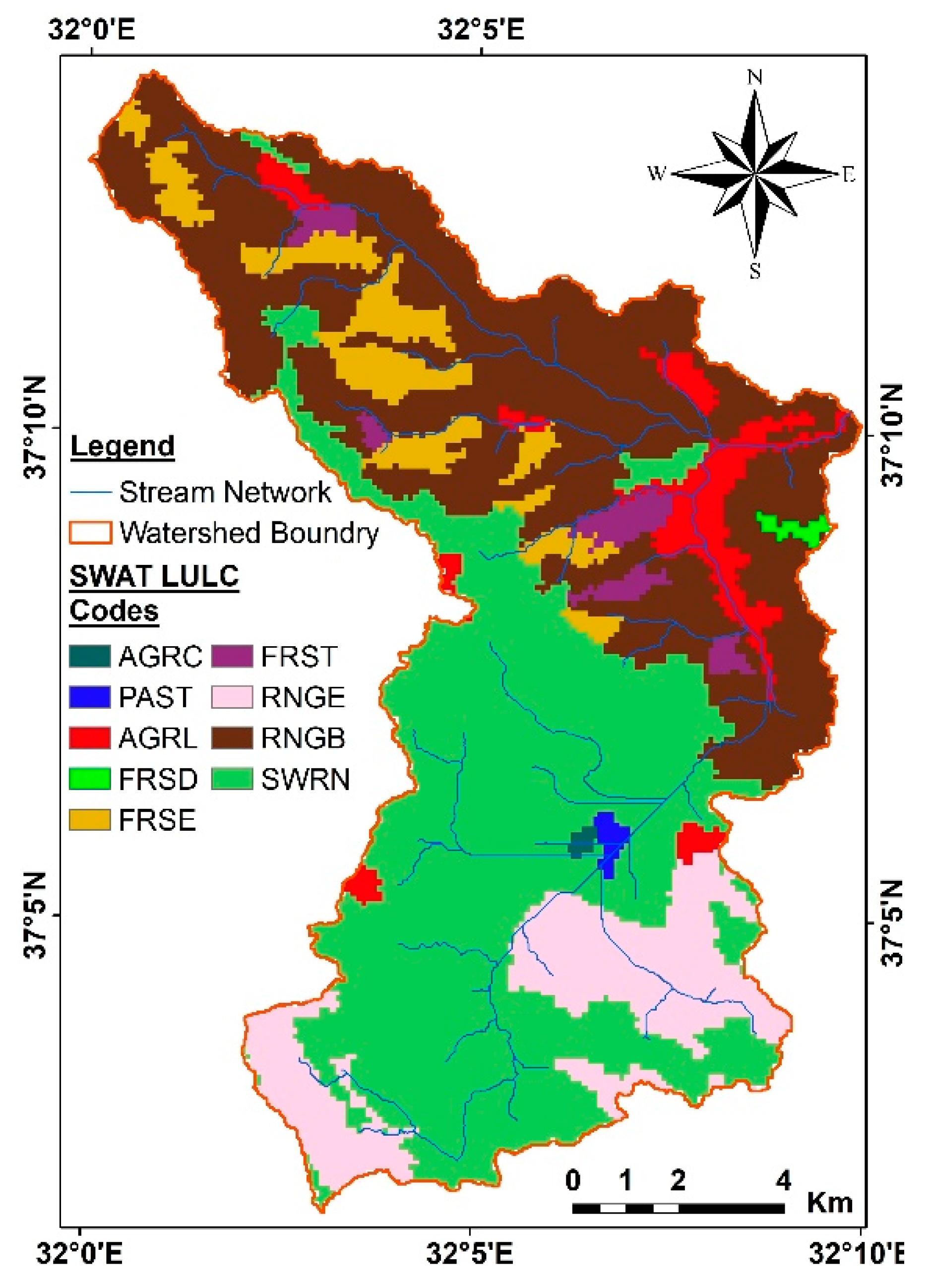
• Land Use/Land Cover (LULC): the LULC map is a significant physical data for the modelling of runoff and infiltration within the SWAT model. The LULC map used in this study is seen in Figure 2. The LULC map used for the SWAT model was denoted from the Coordination of Information on the Environment (CORINE) data. CORINE which was established in 1985 is a program that aims to gather environmental data in Europe, to ensure the coordination of data collection institutions, and to test the reliability of the data obtained. The LULC map is one of the data types produced within CORINE [34].

The LULC of the study area was determined with a view to simulate them by means of the codes of the SWAT model.

SWAT codes and areas of the LULC are given in

Table 1. Soil and water assessment tool (SWAT) codes and areas for LULC.

SWAT LULC Codes	Definition of SWAT LULC Codes	Area (km2)	Area (%)
AGRC	Agricultural Land-Close Grown	0.24	0.16
PAST	Pasture	0.50	0.32
AGRL	Agricultural Land-Generic	7.61	4.94
FRSD	Forest-Deciduous	0.42	0.27
FRSE	Forest-Evergreen	9.46	6.14
FRST	Forest-Mixed	3.22	2.09
RNGE	Range-Grasses	16.32	10.60
RNGB	Range-Brush	52.97	34.42
SWRN	South Western Range-Bare Rock	63.1	41.00

. It may be argued that the dominant LULC in the watershed consists of rocks and plants without woody bodies.

• Soil Types: the soil data was retrieved from the Harmonized World Soil Database v1.2 (HWSD v1.2) data, prepared in collaboration with several organizations, including the Food and Agriculture Organization (FAO) of the United Nations. Since there is no detailed map of soil properties for the study area, HWSD v1.2 data with 30 arc seconds (approximately 1 km) resolution is used. The reference soil depth is 100 cm. The study area was divided into five slope classes (

  Table 2. Characteristics of soil type codes and slope class in the study area.

  	Soil Codes	Area (km2)	Area (%)
  Soil features	I-Lc-E-2b-3114	98.1	63.75
  	I-Be-E-c-3504	43.5	28.26
  	I-Be-c-3093	12.3	7.99
  	Slope Class	Area (km2)	Area (%)
  Slope class of the study area	0-15	29.95	19.46
  	15-24	32.99	21.44
  	24-35	38.00	24.7
  	35-49	32.33	21.01
  	>49	20.58	13.37

  ). According to Table 2, approximately 80% of the study area has a slope class of more than 15%, indicating that the region is quite mountainous.

There are 3 different soil types in the watershed. In the soil codes given in Table 2, the expressions I, Lc, E, Be indicate the available soil types, the other expressions are slope and structure classes. Lithosol (I) is the dominant class among the aforementioned soil types. Lithosols are the rocky soil class, which formed generally as a result of corrosion of rocks found at steep slopes. According to the LULC map, the area having the largest land use of the basin is rocky is in parallel with the fact that the dominant soil class is Lithosol. The soil also includes Luvisol (Lc), Rendzina (E) and Eutric Cambisol (Be) soil types except for Lithosol. There are 3 texture class and 3 slope class in the coding system. Coarse soil, medium soil and fine soil are symbolized by 1, 2, 3 respectively. The slope classes are distinguished: (a) less than 8% slope, (b) between 8% and 30% and (c) more than 30% slope. There are c and b slope classes, 1 and 2 texture classes in the study area.

• Hydro-Meteorological Dataset: precipitation and temperature (max and min) are among the basic climate variables required by the SWAT model. Depending on the PET calculation method used in the model, relative humidity, wind speed and solar radiation may also be necessary. There is no meteorology station with an adequate observation period within the boundaries of the study area. Therefore, the data of the Hadim and Seydişehir meteorological stations operated by the General Directorate of State Meteorology and located near the basin were used. The meteorological data representing the study area were determined by the Thiessen method using the data of these two stations.

At the stage of setup of the SWAT model, while daily temperature (maximum and minimum), precipitation, relative humidity, wind speed, and solar radiation data obtained from Seydişehir and Hadim meteorology stations are used as meteorological data, the streamflow data obtained from D16A115 gauging station operated by the General Directorate of State Hydraulic Works were used (

Table 3. The meteorology and streamflow observation stations used in this study.

Station Number	Station Name	Altitude (m)	Latitude	Longitude
17898	Seydişehir	1129	37°25′36′′ N	31°50′56′′ E
17928	Hadim	1552	36°59′21′′ N	32°27′20′′ E
D16A115	Çarşamba River (Sorkun)	1150	37°10′12′′ N	32°09′44′′ E

). In the set-up, PET was estimated through the Penman–Monteith [35] equation and provided to the SWAT model as input.

According to the observations made in the study area, it was found that the watershed did not experience a significant amount of water loss due to agricultural activities. Since there was no water structure established on the streamflow network, no impact was observed as regulating or changing the streamflow. Therefore, no data were entered into the SWAT model under the heading of management strategies.

In the study, the SWAT model was simulated from 2003 to 2015. The data corresponding to 2003–2005 were used for the warm-up period. While 2006–2011 were used for the calibration period, 2012–2015 were used for the validation period.

2.2.2. Calibration and Validation Process

The SWAT Calibration Uncertainty Programs (SWAT-CUP) is an interface that connects with SWAT models. SWAT-CUP performs sensitivity analysis, calibration, validation and uncertainty analysis in hydrological models [36]. SWAT-CUP consists of algorithms that can solve the different problems that the SWAT model needs for calibration and verification. The algorithms used in the SWAT-CUP program are sequential uncertainty fitting 2 (SUFI-2) [36,37], particle swarm optimization (PSO) [38], generalized likelihood uncertainty estimation (GLUE) [39], solution parameters (ParaSol) [40] and Mark Chain Monte Carlo (MCMC) [41]. However, SUFI-2 is widely preferred among these approaches, since it can provide the widest marginal parameter uncertainty intervals [42]. The successful results were obtained by applying the algorithm to basins with different climatic and physical characteristics [43,44,45]. That is why the SUFI-2 algorithm of the SWAT-CUP for an automatic calibration procedure was used in this study. In SUFI-2, the uncertainty of parameters is described as an interval that corresponds to the uncertainty of all variables. The algorithm takes into account the uncertainties of the parameters, the theoretical substructure of the model, and the measured data. The spread of uncertainty indicates a confidence interval. An interval (95PPU), which consists of the most suitable solutions for SUFI-2 algorithm at a 95% significance level, is achieved as a result. The aim is for the determined confidence interval to include measured data.

The SUFI-2 algorithm takes into account two statistics as P-factor and R-factor in the solution stage. P-factor is the percentage of the actual data covered by 95PPU. R-factor is the thickness of the 95PPU interval. The algorithm operates according to the principle of reaching the lowest R-factor and the highest P-factor. For streamflow estimation, it is recommended to have a P-factor higher than 70% and R-factor around 1 [37]. Theoretically, while the P-factor varies between 0 to 100%, the R-factor takes a value ranging from 0 to infinity. In case the P-factor is % 100 and R-factor is 0, the simulation data and measured data coincide with each other [36].

2.3. Radial Based Neural Network (RBNN)

The ANN contains models with many different configurations and structures. Among these, the RBNN model is one of the models for frequently used in solving physical problems, and yielding highly accurate results [46]. The RBNN which is in the supervised learning class is a feed-forward ANN, similar in structure to the MLP network. The RBNN has a three-layered neural network that consists of an input layer, a hidden layer and an output layer. The network training is carried out in two stages. Firstly, the weights are determined from the input to the hidden layer, and then the weights are determined from the hidden to the output layer. The training/learning is very fast in RBNN models because of simple network architecture. Also, the networks are very good at interpolation. The RBNN model has a few user-defined parameters. This situation is effective for the model to reach a fast solution. The selection of the activation function for the RBNN model, which is frequently used in the non-linear analysis, is also a factor affecting success. Many activation functions, such as linear, cubic, Gaussian, multi-quadratic, inverse multi-quadratic, are used in RBNN models [47], but the most common is the Gaussian function.

$${\varnothing }_j=exp\left[-\frac{{\parallel X-c_j\parallel }^2}{2{\sigma }^2}\right]$$

(2)

where X is the input data of training, c_j is the center value and σ is the bandwidth. RBNNs have the following mathematical representation:

$$y_k=w_0+{\displaystyle \sum }_{j=1}^N{w}_{jk}\times {\varnothing }_j\left(x\right)$$

(3)

where w_jk weight coefficient between the hidden unit j and the kth output unit, ${\varnothing }_j\left(x\right)$ is the response of the jth hidden neuron, and w₀ is the bias constant.

2.4. Support Vector Machines (SVM)

SVM, which has successful applications in the field of machine learning, was first used for classification (SVC) problems, but it was developed in the process and started to be used in the solution of regression (SVR) problems [48]. SVM is capable of making estimations and generalizations for different datasets after learning the training data. Additionally, its operating principle is based on the statistical learning theory and structural risk minimization. The algorithm covered by the model may involve a minimization or maximization purpose, depending on the physical problem. The SVM function can be expressed as,

$$f\left(x\right)={\displaystyle \sum }_{i=1}^N\left({\alpha }_i-{\alpha }_i^{*}\right)K\left(x,z\right)+b_i$$

(4)

where $\left({\alpha }_i-{\alpha }_i^{*}\right)$ is the Lagrange multipliers, K(x,z) is the kernel function, and b_i is the bias. There are two types of SVMs being used for regression, namely Nu-SVR (ʋ-SVR) and Epsilon SVR (Ɛ-SVR). In this study, Ɛ-SVR model was used as the SVR model. There are three parameters that have a direct impact on the success of the model. These are namely the insensitive error term (Ɛ), regularization factor (C), type and parameters of the kernel function. The commonly used kernel functions are linear, polynomial, sigmoid, and radial basis function (RBF). In this study, the RBF was used as a kernel function and this function is denoted as:

$$K\left(x,x\right)=\exp (-\gamma {\parallel x_i-x_j\parallel }^2)$$

(5)

where γ is the kernel function parameter.

2.5. Artificial Intelligence (AI) Models Setup

AI methods are frequently used in hydrological model applications. However, one of the disadvantages of AI models is that the inputs and outputs in the calculation procedure of the model do not contain physical interpretations. The development of effective parameters in the application of AI methods is directly related to the success of the model. In the AI methods, the data during the period from 2003 to 2011 was used in the training process and the data during the period from 2012 to 2015 was used in the testing process.

In this study, meteorological parameters and streamflow time delays are used as input in the RBNN and Ɛ-SVR models which are used to predict streamflow. In the RBNN and SVM models, while precipitation (P_t), lag of precipitation (P_t−1), maximum temperature (T_max), minimum temperature (T_min), relative humidity (RH), wind speed (WS), solar radiation (SR) and lags of streamflow (Q_t−1, Q_t−2, Q_t−3) were used as input parameters, streamflow (Q_t) data were used as output parameter (

Table 4. The structures, inputs and outputs of AI model.

Model Name	Parameters	Parameters Range	Inputs	Output
Radial-based neural network (RBNN)	The number of neurons Spread parameter (σ)	(1–10) (0.01–5)	Qt−1, Qt−2, Qt−3, Pt, Pt−1, Tmax, Tmin, RH, WS, SR	Qt
Support vector machine (SVM)	Regulatory factor (C) Insensitive error term (ε) Kernel parameter (γ)	(1–100) (0.01–0.5) (0.1–8)

).

In the AI models, the most successful model network structure was determined according to the highest Nash–Sutcliffe efficiency coefficient (NSE) value. For the RBNN model, the number of neurons in the hidden layer, which significantly affect the performance of the model, was investigated between 1 and 10, and the spread parameter (σ) was also between 0.01 and 5 using an iterative approach.

In the application of Ɛ-SVR models, many trials were made with an increment of 0.01 in the range of (0.01–0.5) for insensitive error term (ε), an increment of 1 in the range of (1–100) for regulatory factor (C), an increment of 0.1 in the range of (0.1–8) for the radial-based kernel function parameter (γ).

To ensure that parameters with different units are treated equally in a model, the data are rescaled to a certain interval. In other words, the data are made dimensionless. There are no clear rules for a normalization approach in the literature. In this study, before applying the RBNN and ε-SVR to data, the input and output values were normalized between 0 and 1 using Equation (6).

$$X_{norm}=\frac{X_i-X_{min}}{X_{max}-X_{min}}$$

(6)

where, X_norm, X_i, X_min and X_max denote normalized, observed, minimum and maximum values of data, respectively.

2.6. Model Evaluation Criteria

In this study, the performance of models applied in estimating streamflow are evaluated by using mean absolute error (MAE), RMSE, determination coefficient (R²), NSE and percent bias (P_Bias). The equations of these performance indices are available in the literature [22,23,49]. The performance ratings of some statistical indices used are given in

Table 5. General performance ratings.

NSE	R2	PBias (%)	Performance Rating
0.75 < NSE ≤ 1.00	0.75 < R2 ≤ 1.00	PBIAS ≤ ±10	Very Good (VG)
0.60 < NSE ≤ 0.75	0.60 < R2 ≤ 0.75	±10 < PBIAS ≤ ±15	Good (G)
0.36 < NSE ≤ 0.60	0.50 < R2 ≤ 0.60	±15 < PBIAS ≤ ±25	Satisfactory (S)
0.00 < NSE ≤ 0.36	0.25 < R2 ≤ 0.50	±25 < PBIAS ≤ ±50	Unsatisfactory (U)
NSE ≤ 0.00	R2 ≤ 0.25	±50 ≤ PBIAS	Inappropriate (I)

[49,50,51].

3. Results and Discussion

3.1. Results of SWAT

In this study, the study area was divided into 87 subbasins including 845 HRUs, and the SUFI-2 was used to calibrate 20 parameters. The results of analysis obtained using the SUFI-2 algorithm is given in

Table 6. The parameters and values used in the calibration.

Parameters	Parameter Definitions	Range	Fitted Value	Min	Max
R_CN2.mgt	Soil conservation services (SCS) runoff curve number	−0.1–0.1	0.02	−0.07	0.04
V_SFTMP.bsn	Snowmelt base temperature (°C)	−5–5	−0.31	−5.88	1.38
V_ESCO.hru	Soil evaporation compensation factor	0–1	0.10	−0.23	0.58
V_SURLAG.bsn	Surface runoff lag coefficient	1–24	23.78	9.42	26.38
V_GWQMN.gw	Threshold depth of water in shallow aquifer for return flow (mm)	0–5000	−1544.75	−1943.54	2693.54
V_ALPHA_BF.gw	Base flow alpha factor	0–1	0.97	0.34	1.04
R_SOL_AWC.sol	Soil available water storage capacity	−0.1–0.1	−0.01	−0.12	0.02
V_CH_N1.sub	Manning’s value for tributary channels	0.01–1	0.30	−0.46	0.51
V_SMFMX.bsn	Melt factor for snow on June 21 (mm/day-°C)	0–9	7.32	3.70	11.14
V_SMFMN.bsn	Melt factor for snow on December 21 (mm/day-°C)	0–9	7.05	2.57	7.77
V_GW_REVAP.gw	Groundwater revap coefficient	0.02–0.2	0.00	−0.04	0.11
V_REVAPMN.gw	Threshold depth of water in the shallow aquifer for revap (mm)	0–500	83.28	−246.83	251.83
V_EPCO.hru	Plant uptake compensation factor	0.01–1	0.67	0.48	1.44
V_CH_N2.rte	Manning’s value for the main channel length	0–0.3	0.07	−0.12	0.15
V_TIMP.bsn	Snow peak temperature lag factor	0–0.9	0.45	0.06	0.62
V_SNOCOVMX.bsn	Threshold depth of snow, above which there is 100% cover	0–500	232.40	148.19	446.80
V_SMTMP.bsn	Threshold temperature for snow melt (°C)	−5–5	0.78	−7.53	0.83
V_RCHRG_DP.gw	Deep aquifer percolation fraction	0–1	0.73	0.19	0.73
V_GW_DELAY.gw	Groundwater delay time (days)	0–500	162.14	−186.92	271.92
V_SNO50COV.bsn	Fraction of SNOCOVMX that provides 50% cover	0–0.9	0.51	0.28	0.87

. The parameters in Table 6 greatly increased the accuracy of the model. In the calibration, the parameters that represent the evapotranspiration, precipitation, infiltration and underground flow events affecting the streamflow estimation were selected.

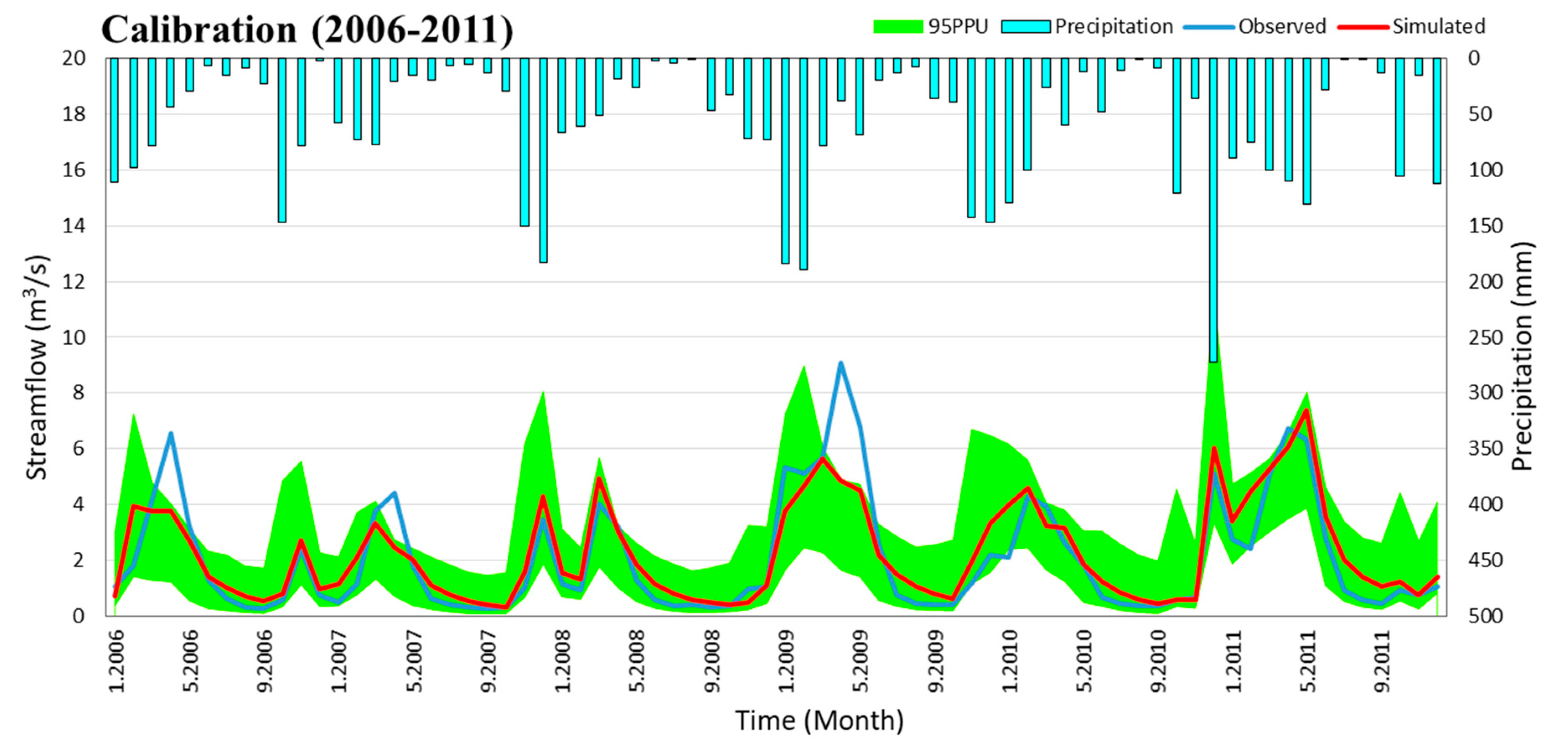
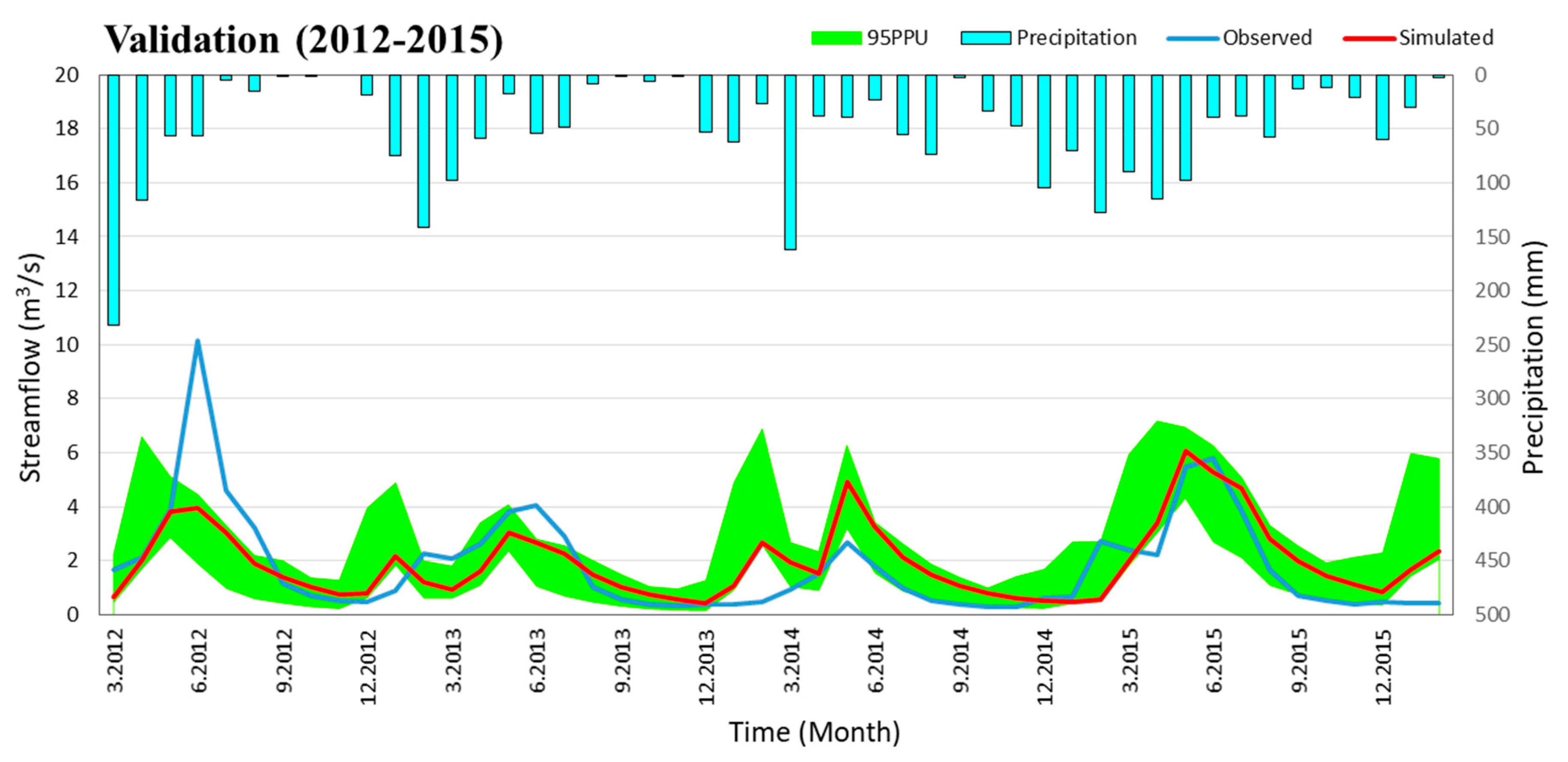
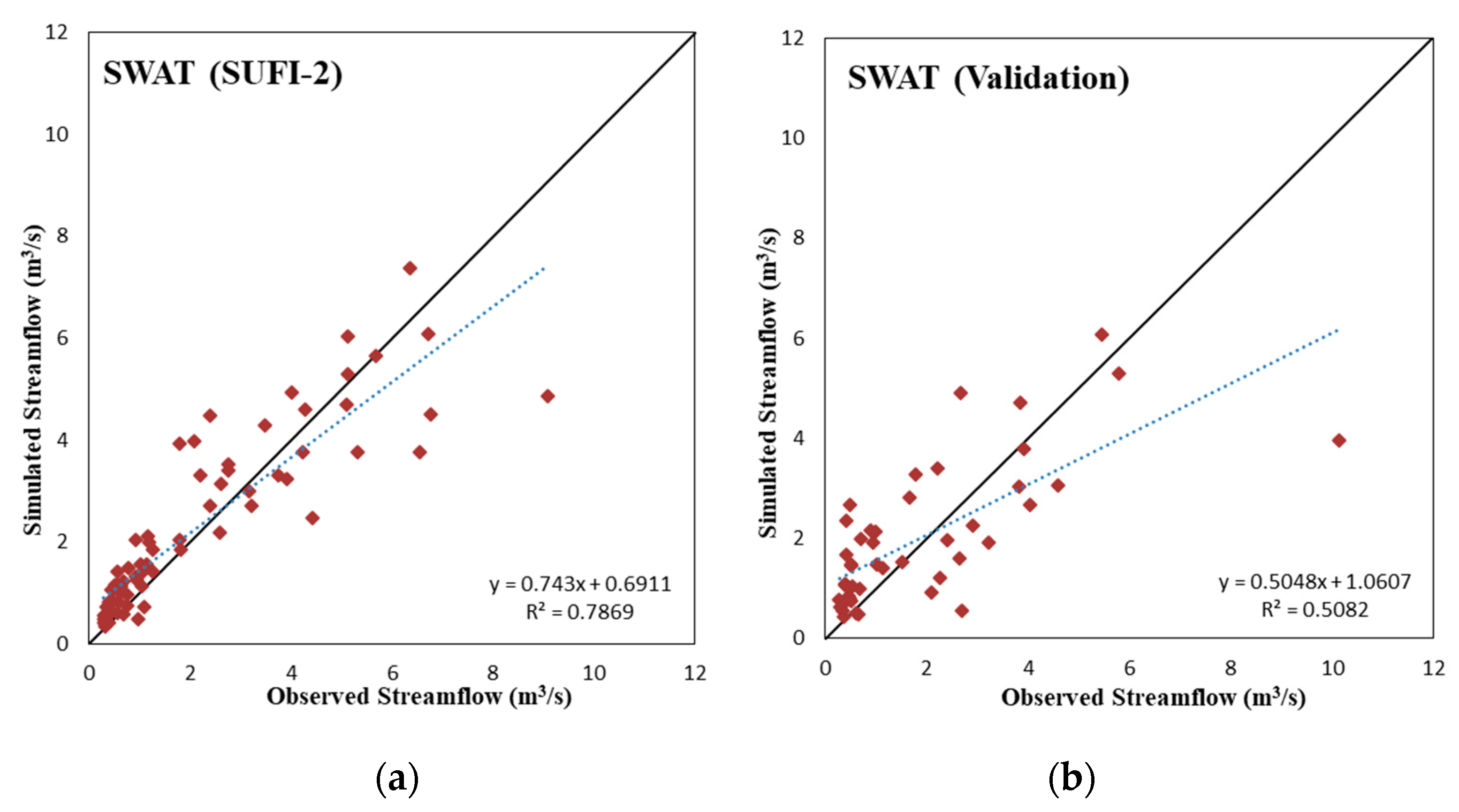
The results of the calibration and validation carried out by the SUFI-2 algorithm of the SWAT model are given in

Table 7. The results of the calibration and validation.

	Calibration (SUFI-2)	Validation
P-factor	0.92	0.63
R-factor	0.94	1.14
R2	0.787 (VG)	0.508 (S)
NSE	0.779 (VG)	0.502 (S)
RMSE (m3/s)	0.962	1.334
MAE (m3/s)	0.645	0.917
PBIAS (%)	−7.562 (VG)	−8.163 (VG)

. According to Table 7, the produced simulation interval covers actual data at a rate of 92% for calibration, and 63% for validation. SWAT seems to yield successful results in view of its performance criteria [49]. According to Table 7, the results obtained for R², NSE and P_Bias in the calibration phase are very good. In the validation phase, NSE and R² results are satisfactory, while P_Bias is very good.

The precipitation data and 95PPU graphs pertaining to the calibration and validation stages of the SWAT are shown in Figure 3 and Figure 4. Although the success of the SWAT was low at peak flow rates, it proved to be successful in estimating lower flow. The climatic and geographic conditions of the watershed led to rapid increases in the flows at times of snow melting, and intense precipitation. However, when the 95 PPU graphs are analyzed, it is observed that the simulation data remain predominantly within the defined confidence interval.

When the development process of the SWAT model was examined, the success achieved in the manual calibration significantly increased as a result of the calibration performed by the SUFI-2 algorithm. At the validation stage, on the other hand, it was observed that the SWAT model showed satisfactory reactions under changing conditions.

3.2. Comparison of SWAT and AI Methods

The parameters of the AI models were determined by trial and error and the most successful network structure was decided according to the highest NSE value in the test period. The most successful network structures for RBNN and SVR models were obtained as RBNN (10, 2, 1, 1) and SVR (10, 10, 0.01, 0.9, 1). The values in the RBNN (10, 2, 1, 1) model represent the number of inputs, the number of neurons in the hidden layer, the value of spread parameter and the output number, respectively. In the SVR (10, 10, 0.01, 0.9, 1) model refer the number of inputs, C, ε, γ and the number of output, respectively.

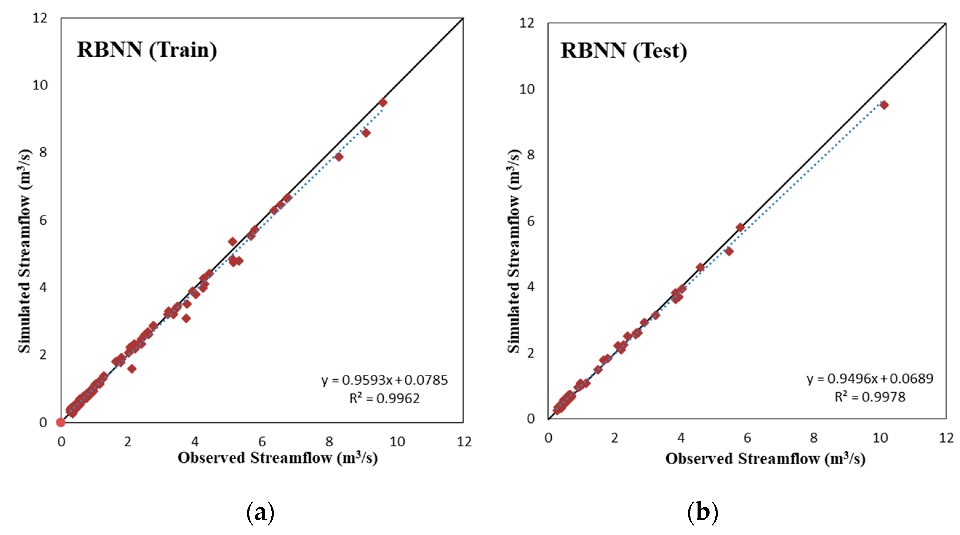
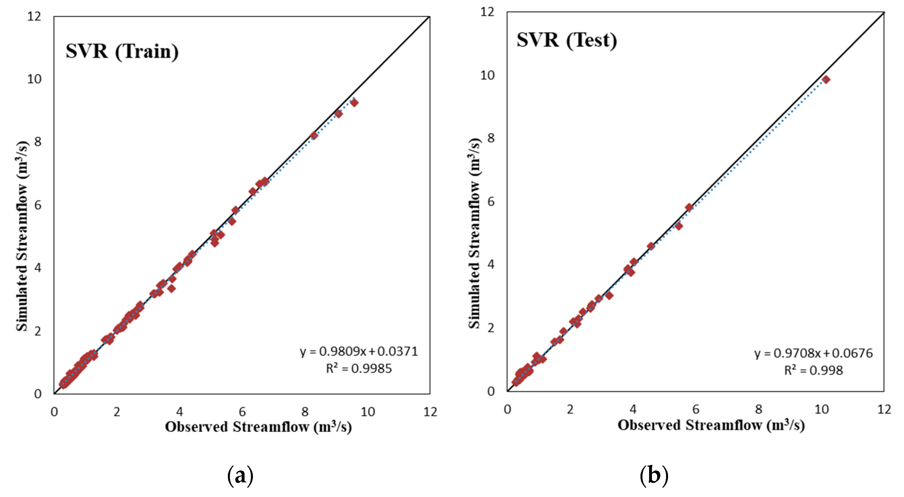
The performance values of the SWAT, SVR and RBNN models are shown in

Table 8. Performance criteria of SWAT model and artificial intelligence (AI) methods.

	Period	R2	NSE	RMSE (m3/s)	MAE (m3/s)	PBIAS (%)
SWAT (SUFI-2)	2006–2011	0.787 (VG)	0.779 (VG)	0.962	0.645	−7.562 (VG)
SWAT (Validation)	2012–2015	0.508 (S)	0.502 (S)	1.334	0.917	−8.163 (VG)
RBNN (Train)	2003–2011	0.996 (VG)	0.995 (VG)	0.149	0.098	0.254 (VG)
RBNN (Test)	2012–2015	0.998 (VG)	0.995 (VG)	0.132	0.079	1.297 (VG)
SVR (Train)	2003–2011	0.998 (VG)	0.988 (VG)	0.089	0.059	0.102 (VG)
SVR (Test)	2012–2015	0.998 (VG)	0.997 (VG)	0.099	0.070	−0.758 (VG)

. According to Table 8, R², NSE and P_Bias values for all models are generally “very good”. However, R² and NSE values have “satisfactory” performance success in the SWAT validation phase. Although the SVR and RBNN models perform very close to each other, the SVR model has achieved a slightly higher success rate than the RBNN model in both the training and testing stages. The meteorological parameters and lags of streamflow (Q_t−1, Q_t−2 and Q_t−3) were used as input variables in the process of creating two non-process based models. The AI models have not included any physical parameters such as DEM, LULC, soil characteristics, and land slope. In AI models, the data were normalized between 0 and 1 to eliminate the unit difference in parameters. Moreover, there is no meteorology station with an adequate observation period within the boundaries of the study area. Therefore, the meteorological data representing the study area were determined by the Thiessen method using the data of these two stations and used as input in the AI models. It is considered that the conditions are effective on the success of the models by reducing the complexity of AI models. The use of streamflow lags in AI models has increased the correlation between input and output. This situation is the most effective factor in the high success of the models. When the SWAT model and AI methods are compared, it is seen that the SWAT model has a lower success than the RBNN and SVR models.

The hydrological model formed using the SWAT model makes possible to comment on numerous hydrologic parameters pertaining to the watershed. In addition, based on the results obtained with the SWAT model, it is possible to undertake analyses that may be useful for different disciplines. The SWAT model can spatially represent a watershed system and hence are capable of predicting flows at various points along a stream network. Although incorporating physical data into SWAT increases the complexity of the model, it creates a model that represents the basin physically well. The SWAT model can also allow a successful simulation of various watershed management strategies for the basin.

AI models must be trained again if streamflow network and meteorological data are revised. Furthermore, AI models cannot be used to predict future conditions if the land use in the watershed changes. Changes of land use cause some changes in water supply and water quality. These changes are a critical issue affecting the hydraulic functions of surface and ground water resources.

In particular, urbanization causes pollution of underground and surface water resources, increase of impermeable surfaces, decrease of groundwater and more flood risk. The change of LULC will have an impact on surface water resources with possible climate change. Therefore, river flows obtained by using existing AI model structures will not fully reflect the effect of the change of land use on the flow. However, these disadvantages of AI models are not available in SWAT models.

Scatter diagrams pertaining to the results attained are shown in Figure 5, Figure 6 and Figure 7.

According to Figure 5, Figure 6 and Figure 7, it is seen that the RBNN and SVR models have less scattered estimates compared to the SWAT model. Also, the slope and bias coefficients of the fit line equation for RBNN and SVR models are respectively closer to the 1 and 0 (an exact line is y = x) and have a higher R² value than those of the SWAT model.

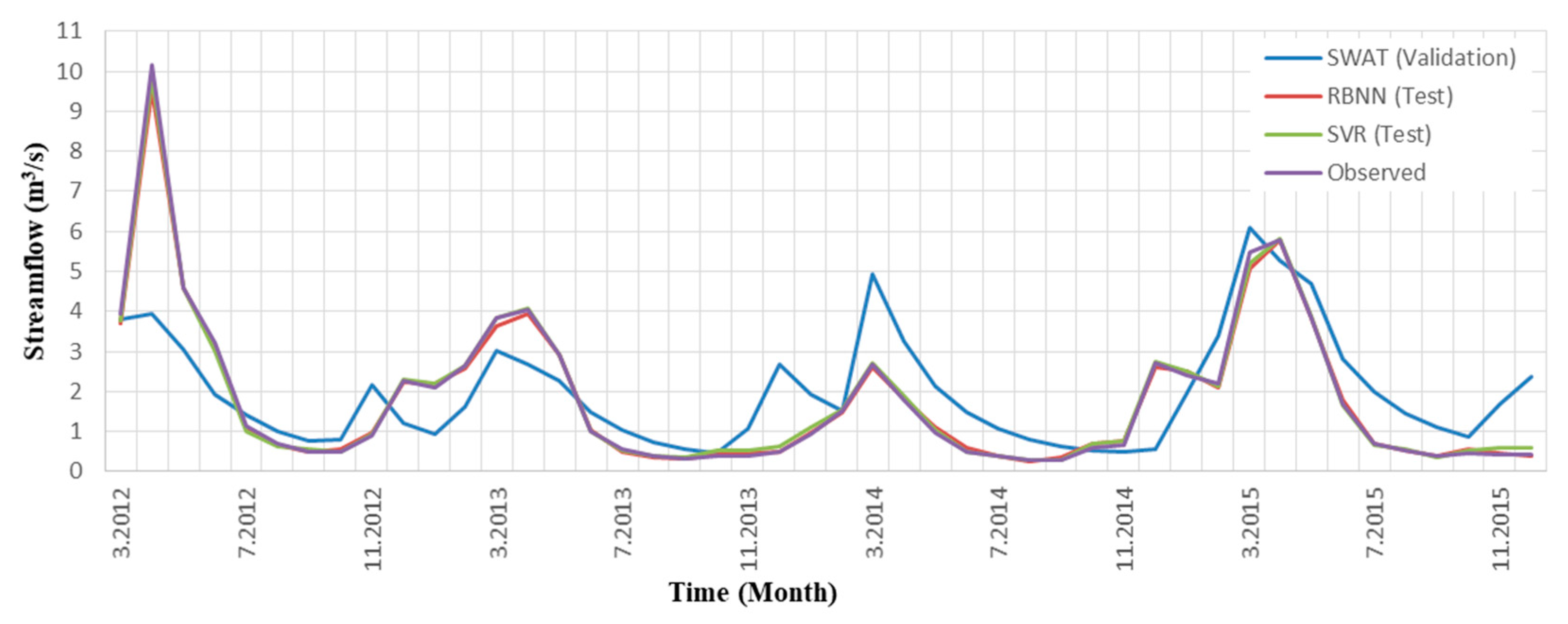
In order to make a comparison between the SWAT model and the AI methods within the time series, SWAT (validation), RBNN (test) and SVR (test) graphs are compared in Figure 8. According to Figure 8, RBNN and SVR models are more successful than the SWAT model for streamflow estimation. According to the time series of the SWAT model in Figure 8, the SWAT model was successful in estimating low streamflow but was relatively unsuccessful in estimating high streamflow.

When similar studies in the literature are examined, it is seen that the results supporting this study are obtained. Demirel et al. [28] reported that ANN was statistically more successful than the SWAT model in predicting daily flow. Jajarmizadeh et al. [29] reported similar results in two models in his monthly flow estimation study with SVM and SWAT. Jimeno-Sáez et al. [52] found that ANN models were successful in predicting higher flows in each case, whereas SWAT was relatively better in simulating lower flows for daily flow modeling in different climate region. Kim et al. [53] used SWAT and two machine learning techniques, ANN and self-organizing map (SOM), for streamflow estimation of the Samho gauging station at Taehwa River, Korea. They found that the machine learning models were generally better at estimating high flows, while the SWAT model was better at simulating low flows.

As can be seen in the process of applying AI methods to the basin, their inability to deliver any physical interpretation regarding the model except for the inputs and outputs, may be considered as the disadvantage of the AI methods. However, AI methods are preferred by different disciplines because of the rapid and accurate results.

Failure to obtain high-resolution data is one of the factors affecting negatively the success of the SWAT model. In addition, the fact that the field observation conducted for the purpose of obtaining information about the watershed was reflected in the model and provided a model closer to reality. Moreover, the fact that the SWAT model was not able to produce successful results in peak flow rates was associated with that the snowmelts could not provide sufficient physical simulation in the modeling for a mountainous region. Due to the lack of a meteorological station in the basin and harsh geographical conditions, some trouble of flow measurements, the hydrological model for the study area made it difficult to establish.

4. Conclusions

In this study, we tested the performance of SWAT, i.e., a physically-based model, for a data-limited and semi-arid headwater of the Çarşamba River. This is part of a mountainous region in Konya Closed Basin. We analyzed the factors that have an impact on the success of the SWAT model. Also, the results of SWAT were compared with the results of ANN and SVM models. While data-driven models give a higher performance on streamflow simulations, they do not provide spatially distributed information over the HRUs which can be required for assessments in agriculture and drought assessments.

• In the SWAT model, the use of the SUFI-2 algorithm for calibration further increased the success of the model compared to manual calibration. According to the results obtained in the validation stage, it is observed that the model produces satisfactory results for changing conditions.
• The SWAT simulations revealed that fast runoff occurs in this mountainous region which can cause a flood risk. The SWAT model performs better during the low flow period as compared to capturing peak flows.
• The comparison of all three models showed that two data-driven models performed better than SWAT. Moreover, the results of SVR model were slightly more successful than those from RBNN.
• The scatter plots show that there was no overfitting problem in the two AI models.
• Although high-accuracy results are obtained with AI models, they only provide discharge outputs. However, the SWAT model is appropriate for solving physical problems related to hydrological processes including snow melt, soil moisture and groundwater. The effect of land cover and land use change on hydrologic fluxes can be assessed by this model too.
• Obviously the quality of the data directly affects the success of the model. The results could improve if there were at least one meteorological station within the catchment.

Future studies on the region should investigate how land uses and vegetation patterns affect water resources using remote-sensing data. Since modeling efforts in ungauged basins is very important for water resources management, satellite products such as the gravity recovery and climate experiment (GRACE), soil moisture ocean salinity (SMOS), moderate resolution imaging spectroradiometer (MODIS) and soil moisture active passive SMAP can offer different hydrologic variables to analyze the catchment fluxes. Global methods such as SCE-UA [54] and CMAES [55] can be incorporated to the SWAT modeling scheme as model calibration can significantly improve the SWAT results.

References

- Sharma, S.K.; Kansal, M.L.; Tyagi, A. Integrated water management plan for Shimla City in India using geospatial techniques. Water Sci. Technol. Water Supply 2016, 16, 641–652. [Google Scholar]
- Anandhi, A.; Kannan, N. Vulnerability assessment of water resources—Translating a theoretical concept to an operational framework using systems thinking approach in a changing climate: Case study in Ogallala Aquifer. J. Hydrol. 2018, 557, 460–474. [Google Scholar] [CrossRef]
- Ayivi, F.; Jha, M.K. Estimation of water balance and water yield in the Reedy Fork-Buffalo Creek Watershed in North Carolina using SWAT. Int. Soil Water Conserv. Res. 2018, 6, 203–213. [Google Scholar] [CrossRef]
- Naschen, K.; Diekkruger, B.; Leemhuis, C.; Steinbach, S.; Seregina, L.S.; Thonfeld, F.; van der Linden, R. Hydrological modeling in data-scarce catchments: The kilombero floodplain in Tanzania. Water 2018, 10, 599. [Google Scholar] [CrossRef]
- Vilaysane, B.; Takara, K.; Luo, P.P.; Akkharath, I.; Duan, W.L. Hydrological stream flow modelling for calibration and uncertainty analysis using SWAT model in the Xedone river basin, Lao PDR. Proc.Environ. Sci. 2015, 28, 380–390. [Google Scholar] [CrossRef]
- Dias, V.D.; da Luz, M.P.; Medero, G.M.; Nascimento, D.T.F.; de Oliveira, W.N.; Merelles, L.R.D. Historical streamflow series analysis applied to furnas HPP reservoir watershed using the SWAT model. Water 2018, 10, 458. [Google Scholar] [CrossRef]
- Swain, S.; Verma, M.K.; Verma, M.K. Streamflow estimation using SWAT model over Seonath River basin, Chhattisgarh, India. Hydrol. Model. 2018, 81, 659–665. [Google Scholar]
- Solomatine, D.; See, L.M.; Abrahart, R.J. Data-Driven Modelling: Concepts, Approaches and Experiences, Practical Hydroinformatics. In Water Science and Technology Library; Springer: Berlin, Germany, 2008; Volume 68. [Google Scholar]
- Kemanian, A.R.; Julich, S.; Manoranjan, V.S.; Arnold, J.R. Integrating soil carbon cycling with that of nitrogen and phosphorus in the watershed model SWAT: Theory and model testing. Ecol. Model. 2011, 222, 1913–1921. [Google Scholar] [CrossRef]
- Iizumi, T.; Sakurai, G.; Yokozawa, M. An ensemble approach to the representation of subgrid-scale heterogeneity of crop phenology and yield in coarse-resolution large-area crop models. J. Agric. Meteorol. 2013, 69, 243–254. [Google Scholar] [CrossRef] [Green Version]
- Abouali, M.; Nejadhashemi, A.P.; Daneshvar, F.; Adhikari, U.; Herman, M.R.; Calappi, T.J.; Rohn, B.G. Evaluation of wetland implementation strategies on phosphorus reduction at a watershed scale. J. Hydrol. 2017, 552, 105–120. [Google Scholar] [CrossRef]
- Vaghefi, S.A.; Abbaspour, K.C.; Faramarzi, M.; Srinivasan, R.; Arnold, J.G. Modeling crop water productivity using a coupled SWAT-MODSIM model. Water 2017, 9, 157. [Google Scholar] [CrossRef]
- Panagopoulos, Y.; Gassman, P.W.; Jha, M.K.; Kling, C.L.; Campbell, T.D.; Srinivasan, R.; White, M.; Arnold, J.G. A refined regional modeling approach for the Corn Belt—Experiences and recommendations for large-scale integrated modeling. J. Hydrol. 2015, 524, 348–366. [Google Scholar] [CrossRef]
- Panagopoulos, Y.; Gassman, P.W.; Kling, C.L.; Cibin, R.; Chaubey, I. Water quality assessment of large-scale bioenergy cropping scenarios for the Upper Mississippi and Ohio-Tennesee River Basins. J. Am. Water Resour. Assoc. 2017, 53, 1355–1367. [Google Scholar] [CrossRef]
- Hallouz, F.; Meddi, M.; Mahé, G.; Alirahmani, S.; Keddar, A. Modeling of discharge and sediment transport through the SWAT model in the basin of Harraza (Northwest of Algeria). Water Sci. 2018, 32, 79–88. [Google Scholar]
- Arnold, J.G.; Srinivasan, R.; Muttiah, R.S.; Williams, J.R. Large area hydrologic modeling and assessment—Part 1: Model development. J. Am. Water Resour. Assoc. 1998, 34, 73–89. [Google Scholar] [CrossRef]
- Abbaspour, K.C.; Faramarzi, M.; Ghasemi, S.S.; Yang, H. Assessing the impact of climate change on water resources in Iran. Water Resour. Res. 2009, 45. [Google Scholar] [CrossRef] [Green Version]
- Bekele, E.G.; Knapp, H.V. Watershed modeling to assessing impacts of potential climate change on water supply availability. Water Resour. Manag. 2010, 24, 3299–3320. [Google Scholar] [CrossRef]
- Setegn, S.G.; Melesse, A.M.; Haiduk, A.; Webber, D.; Wang, X.; McClain, M.E. Modeling hydrological variability of fresh water resources in the Rio Cobre watershed, Jamaica. Catena 2014, 120, 81–90. [Google Scholar] [CrossRef]
- Sisay, E.; Halefom, A.; Khare, D.; Singh, L.; Worku, T. Hydrological modelling of ungauged urban watershed using SWAT model. Model. Earth Syst. Environ. 2017, 3, 693–702. [Google Scholar] [CrossRef]
- Neto, A.A.M.; Oliveira, P.T.S.; Rodrigues, D.B.B.; Wendland, E. Improving streamflow prediction using uncertainty analysis and bayesian model averaging. J. Hydrol. Eng. 2018, 23. [Google Scholar] [CrossRef]
- Tongal, H. Nonlinear forecasting of stream flows using a chaotic approach and artificial neural networks. Earth Sci. Res. J. 2013, 17, 119–126. [Google Scholar]
- Buyukyildiz, M.; Tezel, G.; Yilmaz, V. Estimation of the change in lake water level by artificial intelligence methods. Water Res. Manag. 2014, 28, 4747–4763. [Google Scholar] [CrossRef]
- Temizyurek, M.; Dadaser-Celik, F. Modelling the effects of meteorological parameters on water temperature using artificial neural networks. Water Sci. Technol. 2018, 77, 1724–1733. [Google Scholar] [CrossRef] [PubMed]
- Radzi, M.R.B.; Shamshirband, S.; Aghabozorgi, S.; Misra, S.; Akib, S.; Kiah, L.M. Potential of support-vector regression for forecasting stream flow. Teh. Vjesn. Tech. Gaz. 2014, 21, 1017–1024. [Google Scholar]
- Zhu, S.; Zhou, J.Z.; Ye, L.; Meng, C.Q. Streamflow estimation by support vector machine coupled with different methods of time series decomposition in the upper reaches of Yangtze River, China. Environ. Earth Sci. 2016, 75, 531. [Google Scholar] [CrossRef]
- Hamaamin, Y.A.; Nejadhashemi, A.P.; Zhang, Z.; Subhasis, G.; Woznicki, S.A. Bayesian regression and neuro-fuzzy methods reliability assessment for estimating streamflow. Water 2016, 8, 287. [Google Scholar] [CrossRef]
- Demirel, M.C.; Venancio, A.; Kahya, E. Flow forecast by SWAT model and ANN in Pracana basin, Portugal. Adv. Eng. Softw. 2009, 40, 467–473. [Google Scholar] [CrossRef]
- Jajarmizadeh, M.; Lafdani, E.K.; Harun, S.; Ahmadi, A. Application of SVM and SWAT models for monthly streamflow prediction, a case study in South of Iran. KSCE J. Civ. Eng. 2015, 19, 345–357. [Google Scholar] [CrossRef]
- Noori, N.; Kalin, L. Coupling SWAT and ANN models for enhanced daily streamflow prediction. J. Hydrol. 2016, 533, 141–151. [Google Scholar] [CrossRef]
- Neitsch, S.J.; Arnold, J.G.; Kiniry, J.R.; Williams, J.R. Soil and Water Assessment Tool Theoretical Documentation Version 2009; College of Agriculture and Life Sciences, Texas A&M University System: College Station, TX, USA, 2009. [Google Scholar]
- Tessema, S.M.; Lyon, S.W.; Setegn, S.G.; Mortberg, U. Effects of different retention parameter estimation methods on the prediction of surface runoff using the SCS curve number method. Water Res. Manag. 2014, 28, 3241–3254. [Google Scholar] [CrossRef]
- Elkhrachy, I. Vertical accuracy assessment for SRTM and ASTER Digital Elevation Models: A case study of Najran city, Saudi Arabia. Ain Shams Eng. J. 2017. [Google Scholar] [CrossRef]
- European Environment Agency. Available online: https://www.eea.europa.eu/publications/COR0-landcover (accessed on 2 December 2018).
- Monteith, J.L. Evaporation and Environment. In The State and Movement of Water in Living Organisms; Fogg, G.F., Ed.; Cambridge University Press: Cambridge, UK, 1965; pp. 205–234. [Google Scholar]
- Abbaspour, K.C. SWAT-CUP: SWAT Calibration and Uncertainty Programs—A User Manual; Swiss Federal Institute of Aquatic Science and Technology (Eawag): Dübendorf, Switzerland, 2015. [Google Scholar]
- Abbaspour, K.C.; Johnson, C.A.; van Genuchten, M.T. Estimating uncertain flow and transport parameters using a sequential uncertainty fitting procedure. Vadose Zone J. 2004, 3, 1340–1352. [Google Scholar] [CrossRef]
- Kennedy, J.; Eberhart, R. Particle swarm optimization. In Proceedings of the IEEE International Conference on Neural Networks, Perth, Australia, 27 November–1 December 1995; Volumes 1–6, pp. 1942–1948. [Google Scholar]
- Beven, K.; Binley, A. The future of distributed models—Model calibration and uncertainty prediction. Hydrol. Process. 1992, 6, 279–298. [Google Scholar] [CrossRef]
- Van Griensven, A.; Meixner, T. A global and efficient multi-objective auto-calibration and uncertainty estimation method for water quality catchment models. J. Hydroinform. 2007, 9, 277–291. [Google Scholar] [CrossRef] [Green Version]
- Kuczera, G.; Parent, E. Monte Carlo assessment of parameter uncertainty in conceptual catchment models: The Metropolis algorithm. J. Hydrol. 1998, 211, 69–85. [Google Scholar] [CrossRef]
- Khoi, D.N.; Thom, V.T. Parameter uncertainty analysis for simulating streamflow in a river catchment of Vietnam. Global Ecol. Conserv. 2015, 4, 538–548. [Google Scholar] [CrossRef] [Green Version]
- Notter, B.; Hurni, H.; Wiesmann, U.; Abbaspour, K.C. Modelling water provision as an ecosystem service in a large East African river basin. Hydrol. Earth Syst. Sci. 2012, 16, 69–86. [Google Scholar] [CrossRef] [Green Version]
- Setegn, S.G.; Srinivasan, R.; Melesse, A.M.; Dargahi, B. SWAT model application and prediction uncertainty analysis in the Lake Tana Basin, Ethiopia. Hydrol. Process. 2010, 24, 357–367. [Google Scholar] [CrossRef]
- Hosseini, M.; Ghafouri, M.; Tabatabaei, M.; Goodarzi, M.; Mokarian, Z. Estimating hydrologic budgets for six Persian Gulf watersheds, Iran. Appl. Water Sci. 2017, 7, 3323–3332. [Google Scholar] [CrossRef]
- Moody, J.; Darken, C.J. Fast learning in networks of locally-tuned processing units. Neural Comput. 1989, 1, 281–294. [Google Scholar] [CrossRef]
- Sudheer, K.P.; Jain, S.K. Radial basis function neural network for modeling rating curves. J. Hydrol. Eng. 2003, 8, 161–164. [Google Scholar] [CrossRef]
- Cortes, C.; Vapnik, V. Support-vector networks. Mach. Learn. 1995, 20, 273–297. [Google Scholar] [CrossRef] [Green Version]
- Moriasi, D.N.; Arnold, J.G.; Van Liew, M.W.; Bingner, R.L.; Harmel, R.D.; Veith, T.L. Model evaluation guidelines for systematic quantification of accuracy in watershed simulations. Trans. ASABE 2007, 50, 885–900. [Google Scholar] [CrossRef]
- Van Liew, M.W.; Arnold, J.G.; Garbrecht, J.D. Hydrologic simulation on agricultural watersheds: Choosing between two models. Trans. ASABE 2003, 46, 1539–1551. [Google Scholar] [CrossRef]
- Fernandez, G.P.; Chescheir, G.M.; Skaggs, R.W.; Amatya, D.M. Development and testing of watershed-scale models for poorly drained soils. Trans. ASABE 2005, 48, 639–652. [Google Scholar] [CrossRef]
- Jimeno-Sáez, P.; Senent-Aparicio, J.; Pérez-Sánchez, J.; Pulido-Velazquez, D. A Comparison of SWAT and ANN models for daily runoff simulation in different climatic zones of Peninsular Spain. Water 2018, 10, 192. [Google Scholar] [CrossRef]
- Kim, M.; Baek, S.; Ligaray, M.; Pyo, J.; Park, M.; Cho, K.H. Comparative studies of different imputation methods for recovering streamflow observation. Water 2015, 7, 6847–6860. [Google Scholar] [CrossRef]
- Duan, Q.; Sorooshian, S.; Gupta, V.K. Optimal use of the SCE-UA global optimization method for calibrating watershed models. J. Hydrol. 1994, 158, 265–284. [Google Scholar] [CrossRef] [Green Version]
- Hansen, N.; Ostermeier, A. Adapting arbitrary normal normal mutation distributions in evolution strategies: The covariance matrix adaptation. In Proceedings of the IEEE International Conference on Evolutionary Computation, Nagoya, Japan, 20–22 May 1996; pp. 312–317. [Google Scholar]
- Koycegiz, C. Flow Forecast by SWAT and Artificial Intelligence Methods. Master’s Thesis, Selcuk University, Konya, Turkey, 2018. (In Turkish). [Google Scholar]
Figure 1.
The location map of the study area.
Figure 2.
Land use/land cover (LULC) map of the study area.
Figure 3.
95PPU graph for calibration stage.
Figure 4.
95PPU graph for the validation stage.
Figure 5.
SWAT scatter plots: (a) calibration (SUFI-2); (b) validation.
Figure 6.
RBNN scatter plots: (a) train; (b) test.
Figure 7.
Support vector regression (SVR) scatter plots: (a) train; (b) test.
Figure 8.
Time series of SWAT (validation), RBNN (test) and SVR (test) methods.