Integration of GIS and a Lagrangian Particle-Tracking Model for Harmful Algal Bloom Trajectories Prediction

State Key Laboratory of Marine Geology, Tongji University, Shanghai 200092, China
*
Author to whom correspondence should be addressed.
Water 2019, 11(1), 164; https://doi.org/10.3390/w11010164
Submission received: 7 December 2018
/
Revised: 12 January 2019
/
Accepted: 16 January 2019
/
Published: 17 January 2019
(This article belongs to the Section Water Quality and Contamination)
Abstract
:Harmful algal bloom (HAB) is a major environmental problem in coastal waters around the world. The technologies and approaches for short-term forecasting of the HABs trajectories have obtained increasing attention from researchers. In this paper, we present a straightforward physical-based model based on a non-Fickian Lagrangian particle-tracking scheme for understanding the movement of detected HABs. The model adopts the fractional Brownian motion (fBm) technology, and is coupled with the Delft3D and WRF models and GIS. The fBm based Lagrangian particle-tracking model can flexibly control the scale of the particle clouds diffusion through Hurst value, which can be used to account for uncertainties and adjust for better representing the trajectories of HABs. Simulation results demonstrate that the presented model can successfully predict the trends and the main features of red tide drifting. The developed simulation tool enables users to create the model configuration, manage data inputs, run the model, and generate model maps and animations within a GIS environment. It is believed that the model and the tool outlined herein can be very useful for rapidly evaluating potential areas at risk from the HABs events.
1. Introduction
As is known, HAB is a predominant oceanographic phenomena in coastal waters. Over the past few decades, known as red tide, blue-green algae or cyanobacteria, HABs have been increasing in frequency worldwide and have posed negative impacts on human health, aquatic ecosystems and the economy [1,2,3]. These challenges motivate the development of many new technologies and approaches for bloom detection, monitor, forecasts, and assessment. Although the bloom-triggering conditions and blooms detection are important targets in HAB studies, the capacity to predict the HAB trajectories in a temporal window of a few days has been considered as the key topic in recent years. The short-term HAB trajectories’ forecasts can provide early warning services and enable decision-makers to respond rapidly and minimize the environmental and economic impacts shortly after the HAB events.
HABs are complex processes that require multidisciplinary study and methodologies. All of the methodologies mentioned in the literature can be grouped into three major categories, namely remote sensing, field observations and measurements and numerical modeling [4,5]. Although remote sensing has demonstrated the ability to detect and monitor surface HABs; however, it also presents some significant drawbacks. The method is inadequate to identify low biomass (densities) blooms. Moreover, satellite ocean color images are limited by clouds and spatial resolution. In situ observations and measurements overcome some of the limitations of satellite system; however, in situ data are typically scarce and often lack spatial resolution, and therefore significant cost and inefficiency [3,4,6]. Most of all, both remote sensing and in situ observation present limitations in providing HAB trajectories’ predictions. Given the constraints of satellite imagery and field observations’ methods, an alternative solution is to adopt numerical modeling technique to meet the demands of forecasting the spatial and temporal evolution of HABs [7]. Compared with the observational and remote sensing approaches, numerical modeling can provide a general understanding and trends of the transport and dispersion of HABs at high spatial and temporal scale with a significantly lower cost.
In the past few decades, researchers have proposed different modeling approaches to simulate HAB trajectories. McGillicuddy reviewed many numerical modeling developments related to HAB simulation [8], and Davidson et al. identified a range of modeling methodologies and their strengths and weaknesses [6]. These developed models vary significantly in complexity and on the processes they address, including the straightforward physical-based models, as well the ecosystem based models coupling physics with biological processes. Because of requiring only a few inputs, the physical-based models are considered as the most effective and practical method. By contrast, most of the ecosystem based models present enormous difficulties beyond physics, which generally require a lot of inputs, making the models fuzzy and difficult to implement [6,7,8]. Lynch et al. pointed out that simulations are typically chosen to fit field problems and available data [9], and some valuable research works have highlighted that the physical-based Lagrangian particle-tracking model (LPTM) are sufficient to predict HAB trajectories [8]. Lagrangian based models do not incorporate the processes of biological growth or decay of a bloom, recommending the framework are especially suitable when physical processes dominate over biological ones [6]. In recent years, the LPTM method has been extensively applied and previously shown to successfully simulate transport of pollutants in water pollution studies [10,11,12,13,14,15,16,17].
Although a number of Lagrangian based models have been proposed to estimate the trajectories of HABs, there is still a need to continuously formulate new modeling approaches for better understanding and predicting the movement of HABs. Theoretically, the Lagrangian based method is accomplished with a random walk technique, using to simulate the turbulent diffusive transport [18]. In most traditional Lagrangian based modes, the random component implemented is Fickian (e.g., white noise) modeled as Brownian motion [17,19]. Brownian motion, a continuous-time random walk, is widely used in particle tracking models to predict pollutants dispersion in oceanic flows [20,21]. However, some studies have demonstrated that non-Fickian diffusion is frequently observed in pollutant diffusion processes due to the long-range correlations (Lagrangian memory effects) in velocity flow fields. Traditional particle-tracking techniques can’t model the non-Fickian diffusion process using uncorrelated random displacements drawn from a Gaussian probability distribution [22,23]. Sayol stated that a non-Fickian distribution for the random term is recommended [17]. Thus, a technique that employs fractional Brownian motion (fBm) has been suggested as a possible stochastic process for the simulation of non-Fickian diffusion within a particle-tracking model [22,23,24,25]. Recently, the fBm method has been adopted to simulate the dispersion of an oil spill on the water surfaces [21]. Therefore, one main purpose of this study is to adopt the fBm method to present a non-Fickian Lagrangian particle tracking scheme coupled with the operational models for investigating the HAB movement on the coastal waters surface. Furthermore, in order to make the presented model easily deployable and adaptable to various oceanic areas, the present work also concentrates on the integration method of linking the fBm model and the operational forecasting models (atmospheric and hydrodynamic) together. Additionally, HABs’ drift is typically spatial and temporal variations, and thus the spatial dimension is essential in HABs transport and dispersion modeling. In a given emergency situation, researchers and decision makers need to quickly obtain spatial and visualized simulation results. However, there are fewer applications and studies about the development of visualization and spatial analysis tools coupled with the fBm based LPTM for HAB transport and dispersion simulation. Moreover, most HAB trajectories modeling rely on an experienced team of scientists or model developers to construct and run the simulation because of model runs with the complicated and unfriendly user interface, which may limit the widespread application of such model and simulation tool. In this context, the efforts compiled in the present work also focus on seamlessly integrating the fBm based LPTM with Geographic Information System (GIS), providing a user-friendly and geographically referenced environment for model runs, results visualization and spatial analysis. In summary, the key goal of this study is to present a GIS-based modeling framework, which gives decision makers an opportunity to rapidly obtain visualized predictions and evaluate potential areas at risk from the HAB events, and therefore respond rapidly and revise their strategies for emergency HAB events.
The remainder of this paper is organized as follows: Section 2 gives a general description of the mathematical equations of the fBm based particle-tracking diffusion model. Section 3 outlines the general framework of the model and GIS integration, and introduces the development of the GIS-based simulation tool. Several numerical experiments were conducted to evaluate the model and show the applicability of the GIS based simulation tool in Section 4. Section 5 summarizes the conclusions, together with some suggestions for further work.
2. Model Descriptions
In principle, the HABs are regarded as an instantaneous release and considered as a set of independent and passive particles in a Lagrangian framework. The movement of particles on coastal water surfaces is forced by advection/diffusion mechanisms, calculating the trajectory of each particle individually. The advective velocities generated by hydrodynamical and meteorological models are used to force the model. The diffusion is regarded as a stochastic process, simulated using random walk approaches such as regular or fractional Gaussian random walk.
In this study, winds and currents data obtained from either estimates generated from the implemented operational models or user defined velocities constants in space and time were used to drive the fBm based LPTM model runs. The operational models can be integrated with a LPTM in the form of offline or online linkage approach. A major benefit of offline linkage approach is the possibility of making use of available operational models outputs for running LPTM experiments, avoiding computational costs of re-running the physics coupled to the Lagrangian module [7,16]. Secondly, it can also provide a convenience of developing an interactive GIS environment to run an LPTM. Furthermore, offline simulation uses winds and currents from the operational models running at different sites, making the LPTM easily deployable and adaptable to various oceanic areas. Considering the above-mentioned factors, the study adopts the offline linkage approach.
In this study, the hydrodynamics model Delft3D, developed by Delft Hydraulics (Delft, Netherlands) was adopted to forecast current velocities with a 1 km horizontal resolution. The Delft3D hydrodynamic model was developed with a set of programs capable of simulating flows in surface water bodies. The Delft3D-Flow model solves the Navier–Stokes equations for an incompressible fluid under the shallow water, which can be used to predict the flow in shallow seas, coastal areas, estuaries, lagoons, rivers and lakes [26]. A uniform mesh grid atmospheric model, Weather Research and Forecasting Model (WRF), was used to calculate the wind U and V components at 10 m above the water surface in the x- and y-directions, with a 5-km grid spacing. The WRF model is a new-generation mesoscale NWP system that solves the nonhydrostatic compressible Navier–Stokes equations to serve both operational forecasting and atmospheric research needs, which is suitable for a broad range of applications and widely used by both operational and research communities [27,28]. Both the Delft3D and WRF models routinely undergo strict validation and calibration procedures, ensuring to provide a reliable forcing data for the fBm based LPTM.
The implicit assumption made in this work is that the model is a two-dimensional (x and y) Lagrangian model, which assumes that particles are only released into the surface layer and does not take into account the vertical migration. The particles have passive transports that are advected in two dimensions according to coastal surface currents and winds fields, and plus a stochastic term to represent unresolved turbulent motions. In this approach, a particle cannot be subdivided and moves individually on the water surfaces without interaction each other. In a simulation, if a Lagrangian particle reaches the coastal line or the boundary of the model domain, it rebounds back to a previous location and keeps on taking further part in the simulation. Additionally, the model strongly depends on the initial position of HABs. Thus, the evolution of the HABs location is obtained by solving the equations in the following section under an assumption of knowing the HABs’ initial location.
In a general LPTM scheme, the new position of a single particle at each time step t + △t is calculated using the following equations:
where represents the particle position at the current time step, and is the Lagrangian time step. The advective velocities is calculated as the linear combination of currents and winds velocities, expressed as Equation (2). The is the user-defined wind transport coefficient. To obtain the velocity fields at the Lagrangian time step, linear temporal interpolation of currents and winds velocities’ fields is carried out according to Equation (3), where U1, U2 and V1, V2 are the pre-calculated velocities of winds or currents in x- and y-directions, respectively, at t1 and t2 computational time steps. The is the particle displacement due to turbulent motion which is simulated according to the based fBm Equation (4) and its derivative formulation [22,23,24,25], where (t) is a continuous function with zero-mean increments and variances, which scale as ~t2H, and H(0 < H < 1) is called the Hurst parameter. is a gamma function introduced to ensure that the fractional integral becomes an ordinary integral when H + 1/2 is an integer [21]:
The fBm is a generalization of regular Brownian motion. The main difference to the regular Brownian motion is that the fBm is characterized by the Hurst exponent, which can control the scale of diffusion. It should highlighted that the main focus in this paper is to employ the fBm technique in a Lagrangian framework, rather than investigating and deriving the algorithm of the fractional Brownian motion itself. A good overview about this comprehensive theoretical work is given in [22,23,24,25].
3. GIS-Based Simulation Tool
3.1. The Conceptual Framework of the Model and GIS Integration
Because of the spatial nature of model outputs, the geospatial techniques such as GIS may facilitate visualization and identification of spatial distributions of simulation results, and therefore the use of GIS in conjunction with modeling has become increasingly important in many geoscience fields. The versatility of GIS to act as a data pre- and post-processor as well as its ability to act as an effective data management and visualization platform and its capability to perform further spatial analyses [29], which makes it an ideal platform for evaluating the spatial information of HAB transport and distribution. In this work, our objective is to combine modeling and GIS technologies to develop a simulation tool that is able to run the fBm based LPTM and generate intuitive and easily interpreted outputs in a GIS environment.
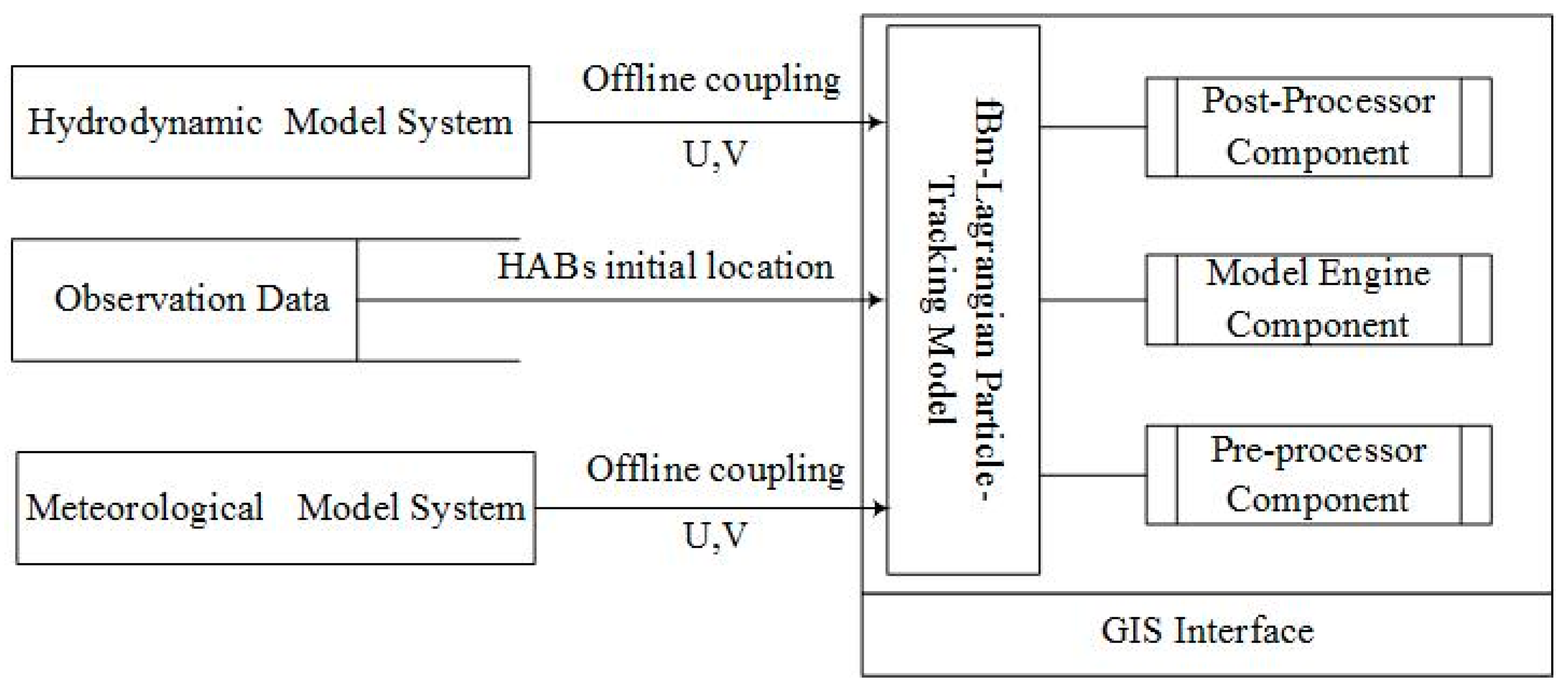
The framework chosen for achieving the GIS-based HABs transport and dispersion simulation tool includes several components, as shown in Figure 1: (1) the interactive GIS interfaces for simplifying the complicated modeling operation, and ensuring the entire modeling process is user-friendly enough to be operated by non-professional users; (2) the pre-processor component includes functionalities necessary for the model inputs preparation; (3) the model engine component provides the ability to perform calculations and run model simulations for obtaining the current bloom locations, future bloom locations, and areas of impacts; and (4) the post-processing component is designed to generate visualization maps and animations. The following sections give a brief description of the specific features supported by the above-mentioned components. The details of the software developing specifications and implementation workflow have already been presented in our previous work [30].
3.2. GIS Interface
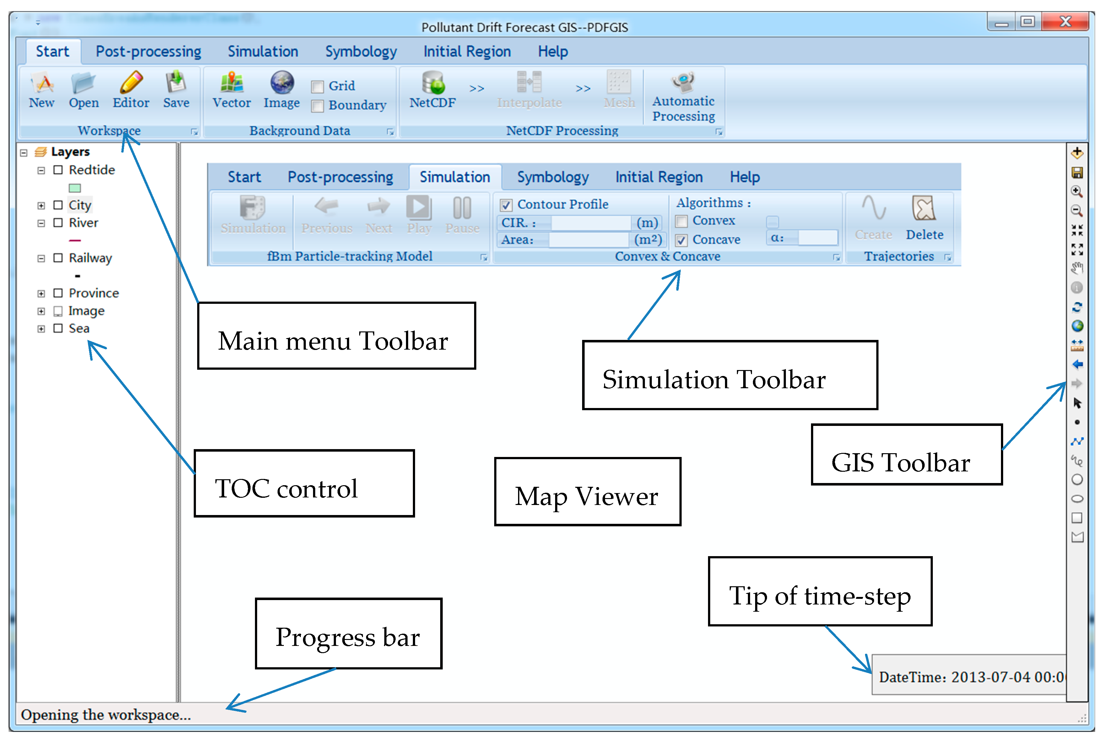
The GIS interface was built upon ESRI ArcGIS Engine functions using Visual C# .NET and C++ programming language. For providing convenient operations, the graphical user interfaces (as shown in Figure 2) was designed as a familiar primary interface similar to most desktop GIS programs, which allows a user without any technical training to run HAB simulation via easy-to-use interfaces. The interfaces mainly consist of a ribbon-style main menu, a map viewer window, a table of contents control (TOC), a progress bar and a toolbar, as well as a simulation workspace management window form. The map viewer window is the main visualization element, used to display the spatial distribution of simulation results and relevant background marine and land data. The simulation workspace interface allows users to quickly and easily define or adjust the basic modeling parameters, consequently simplifying the setup and application of the model; the workspace interface also is used to manage the simulation project information such as a project name, created and latest modified times and the directory storing the project file. Although the HAB simulation process can be divided into four steps, namely inputs preparation, operational model outputs’ pre-processing, model computation, and model results processing and visualization, the GIS interfaces integrate them closely under a pre-defined workflows, and thus the simulation can be semi-automatically executed with few user operations.
3.3. Pre-Processor Component
The pre-processor component reformats the operational model outputs and prepares necessary inputs for driving the model runs, including the following pre-processing steps: (1) Firstly, forcing data need to be converted from NetCDF format to a readable data format. Using the NetCDF library for .NET (nt.dll), we wrote a NetCDF Data Reader component for parsing the data values at the mesh nodes. (2) In the next step, an interpolator component was developed to interpolate operational models forecasts value temporally for generating the velocities of surface currents and winds at the simulation interval according to Equation (3). The interpolation data were written into a set of a specifically formatted text files that can be easily accessed by further analysis and visualization programs. (3) Then, a mesh generator program was designed to generate computational mesh of the model in the form of vector polygon shapefiles. Therefore, the generated mesh-grid shapefiles can be loaded into the map viewer for identifying a particle contained in an individual mesh element during model calculations. (4) Finally, the modeling approach requires the input of one or several polygons in the form of shapefile. These polygons are known as the initial location of HABs. In the developed GIS tool, we provide an editor tool for creating such polygons. Similarly, the geospatial pre-processing of initial release location can also be performed in other GIS platforms (e.g., ArcGIS Desktop software (ESRI, RedLands, CA, USA)).
3.4. fBm Based LPTM Engine Component
The pre-processing of forcing data has been executed to completion, and then it needs to define some basic coefficients for performing model calculations. The coefficients in the model are listed in Table 1. Settings can be saved and reused in order to retrieve simulation runs.
Once the parameters have been defined, the calculations can be executed in order to generate time-series distribution of particles. The following calculation processes were involved: (a) HABs initial release domain discretization for calculating initial positions (latitude and longitude) of particles; (b) topology calculations for identifying each particle in the mesh cell belongs; (c) diffusive component calculation; (d) particles feature location estimation; and (e) contour profile of particle clouds (HABs shape) and areas calculation. Except for the initial position calculation, other calculations need to be performed at each time-step.
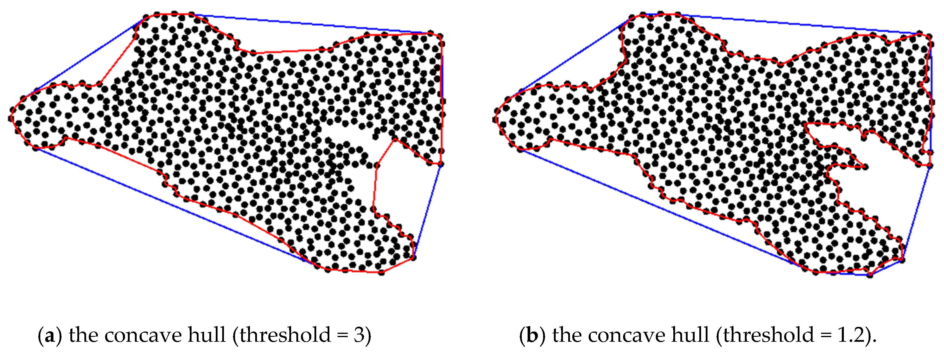
The first two calculation steps are spatial operations that can be performed using ArcGIS Engine functions. Firstly, depending on the geometry of the initial domain and the pre-defined particles count, the initial positions of particles in a given region are assumed evenly distributed within the polygons. Then, it needs to determine a particle contained within which one mesh cell by using point-in-polygon topology operations, and adopting the corresponding value to calculate the advective components. The diffusion components are computed according to Equation (4) and its derived equations. Obtaining the advective and diffusion displacements, the model can define and record each particle location at every computational time-step. The lastly step, the ‘α-shape’ algorithm is employed to construct the concave hull of scatter particles. The generated concave hull is defined as the potential areas impacted by the HABs. As shown in Figure 3, the concave hull is more suitable to characterize the geometrical shape of scatter particles than the convex hull. Comparing Figure 3a and Figure 3b, it clearly illustrates that the algorithm can capture the exact geometrical shape of a dataset’s surface through an optimal threshold value. Furthermore, once the model has completed calculations at a particular time-step, the point-based calculation results are then written to an output file. Additionally, a particle movement was tracked to generate its trajectory. A simulated trajectory allows for tracing the probability pathway of a specified particle along the coastal water surfaces at each time-step.
3.5. Post-Processor Component
The post-processor component was designed to provide efficient post-processing methods that would visualize the outputs for identifying and evaluating potential HAB areas and comparing them with field data for model simulation validation. In the procedures, the results were displayed in the map viewer in two graphical formats. On the one hand, the program generates vector layers for operational models’ grid points (i.e., currents and wind layer) according to the pre-processing results, and renders the layers with arrows that indicate the currents and winds direction and magnitude. On the other hand, the particles’ movements and the corresponding tracking trajectories and concave hull are displayed as graphical element layers, which can have a different spatial and temporal extent at each time-step.
4. Results and Discussion
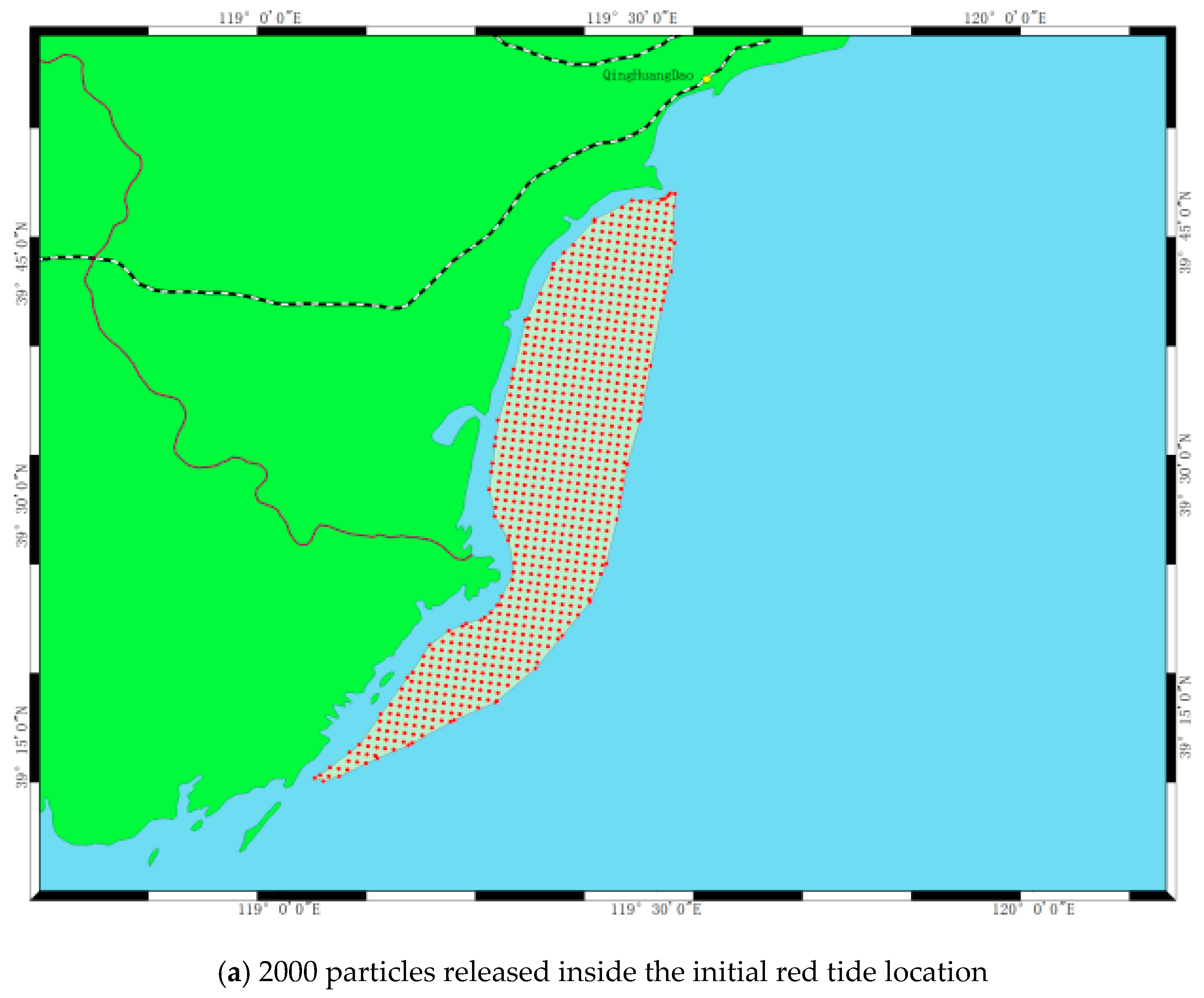
Several model runs were performed in this case study, in order to demonstrate the abilities of the model and the developed GIS tool. Considering the availability of field data to describe the HABs, a harmful algae bloom commonly called red tide, which occurred near the Qinhuangdao coastal water was selected for the sample application. Initially, the red tide was represented as 2000 particles, using the fBm based LPTM to track the trajectories at 30 min intervals, starting from the known position at 10:00:00 a.m. on July 2th 2013 (as shown in Figure 4a), to the locations at 3:00:00 p.m. on July 4th 2013. The value of M was given a value of 24,000 that is much larger than the total steps of computation time. The Hurst takes values of 0.76 and 0.5 in different model runs, respectively. The initial location of HABs and validation of the transport and dispersion of particles was made based on datasets from coastal monitoring programs, provided by the Marine Environmental Monitoring Center of Hebei Province. The geospatial data pre-processing of observation data sets were performed in ArcGIS Desktop software (ESRI, RedLands, CA, USA) to provide the inputs for the fBm model runs. Hourly currents and winds from Delfd3D and WRF are used to force the model. Because the simulation tool accepts the netCDF data as forcing inputs, a MATLAB (MathWorks, Natick, MA, USA) program called ‘vs_trim2nc.m’ was used to convert the Delft3D trim NEFIS file into a netCDF file.
When a red tide drifting was simulated, a set of 2000 particles was placed inside the initial red tide location, as shown in Figure 4a. The fBm based LPTM computes the trajectory of each particle and the concave hull of particles (red tide area) as described in the previous sections during the 53 hours of simulation. When a simulation was done, the time-varying positions of simulated particles were visualized in form of a continuous and automatic animation.
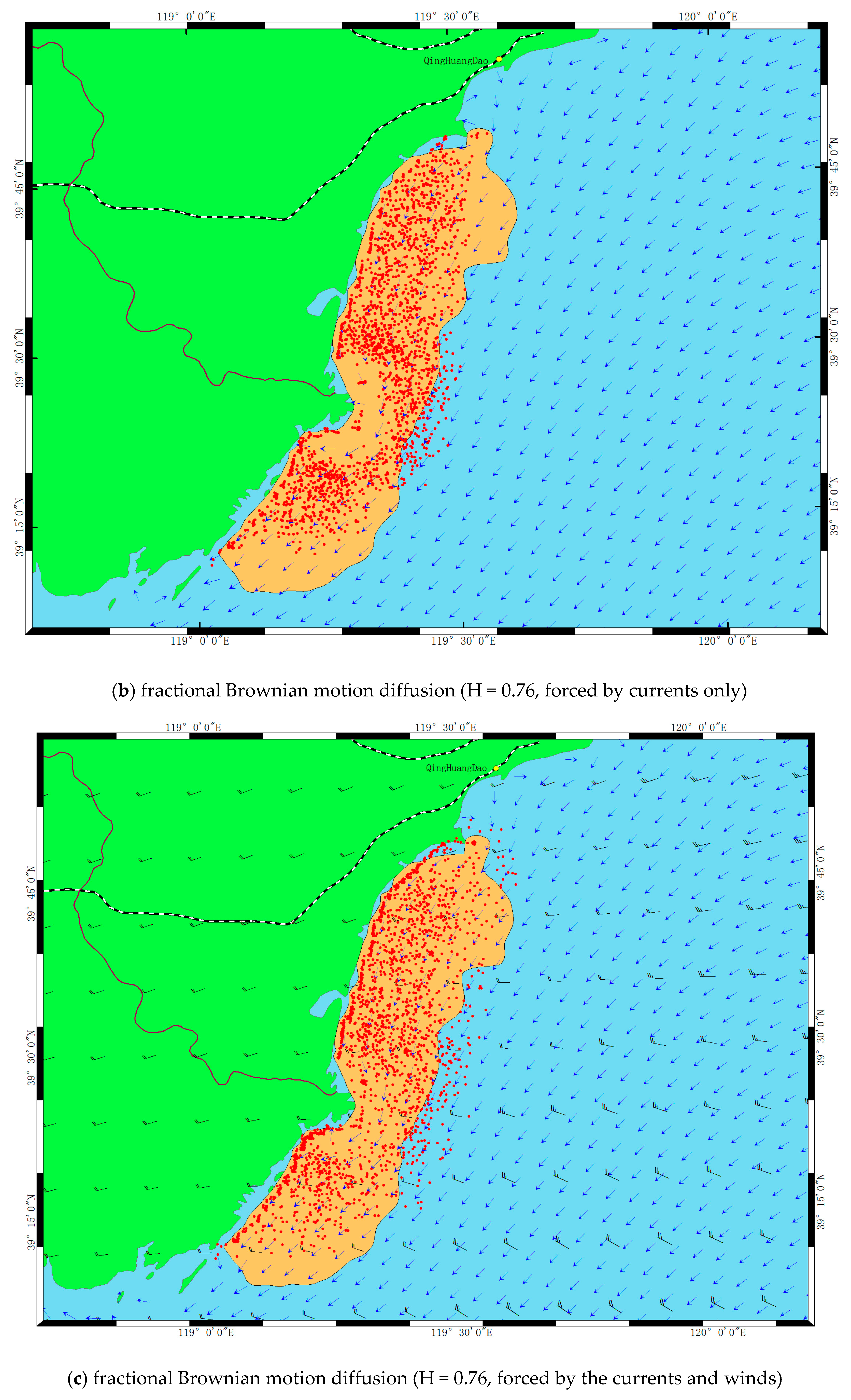
To evaluate the impact of physical forcing factors on the control processes of the HAB transport, two model runs’ scenarios with and without surface winds forcing were performed with the same Hurst value (H = 0.76). In the first experiment, the particles were solely forced by surface currents under the no-winds condition. A second experiment was carried out with the combined effects of the surface currents and winds. The effects of physical factors on mechanical spreading are illustrated in Figure 4b,c, which indicate the difference of the particle clouds diffusion undergoing the fractional Brownian motion diffusion simulation with different forced conditions. The simulations show that the surface current fields have a dominant impact on the particle trajectories. However, as the fact that HABs is directly exposed to the water surface, these numerical experiments also showed that the simulation results with and without wind conditions differed slightly.
We mentioned in the introduction that the fBm based Lagrangian particle tracking method (H > 0.5), versus regular Brownian motion method (H = 0.5), has the advantage of controlling the scale motion of the diffusion clouds and best approximates movement of particles. To test this assumption, we made another model runs to verify the effectiveness of LPTM based on regular and fractional Brownian motion, respectively. Figure 4d presents the particle clouds undergoing regular Brownian motion (H = 0.5) under the same forcing conditions as the second experiment mentioned before. Comparing Figure 4c and Figure 4d, it shows that the results obtained from two kinds of numerical model differed fundamentally.
Considering observation data sets were available in this case study, the authors evaluated the accuracy of the simulation in two ways. On the one hand, a quantitative area comparison between the model simulations and the in situ observations were performed (Table 2). It is evident that the area of the concave hulls generated by the fBm model is larger compared with the regular Brownian motion method, and the one based on fBm is closer to the observation data sets. On the other hand, the spatial distribution of particles can also be used to evaluate the simulation. Although the areas of the concave hulls in Figure 4b,c are all closer to the observations, however, the simulation results clearly illustrate that the distribution of particles generally covers the observations and the shape of the trajectory is better represented based on the combined effects of the surface currents and winds forcing. This means that the wind forcing is also an important factor in determining the transport pathways of HABs. In these simulations, we noted that once surface floating material leaves its place of origin, its spatial distribution is generally controlled by currents and winds. Furthermore, the simulation results also reveal that the fBm based LPTM has a flexibility to control the particles diffusion through Hurst value, which can be used to account for the uncertainties of HABs transport and dispersion. Meanwhile, it also indicates that the larger H adopted, the larger diffusion range is presented. However, because the Hurst value makes the scale of the particle clouds exponentially diffusion at each time-step, we noted that there is a noticeable increase in the spreading rate of the particle clouds with time raised in the case study. Therefore, it is beyond the ability of the Hurst value to describe the uncertainties in a long-term simulation. We hence state that the fBm based LPTM seems legitimate during the early stage (in a temporal window of a few days) of HABs drifting simulations. As it is known that most HABs are usually short-lived, typically lasting a few days [31], we thus conclude that the model can be used to simulate the entire duration of HABs event.
Because the predictions being subject to multiple sources of uncertainty, we note that a simulation with fBm based LPTM still shows differences between observations and model results. On the one hand, the input forcing fields used to drive the model provided by numerical models have their own uncertainties. Additionally, the initial HABs’ location and validation data collected from field measurements or remote sensing images are an estimation of the actual position of the HABs, which may contain location errors and directly affect the HABs drift forecast accuracy and the comparisons. For these reasons, the performed simulations in this case study can be acceptable with respect to the uncertainties. It also demonstrates that the proposed method can be a feasible alternative to simply simulate the bloom dispersion and transport in a non-biological way with only fewer inputs. However, we should point out that one drawback of LPTM is that it requires a large number of particles to accurately describe the trajectories, which requires abundant computer resources and might become a challenge when working in larger domains for a multi-day transport simulation.
5. Conclusions
The presented fBm based LPTM is a physical process model without involving any biological processes, which works coupled with existing hydrodynamic and atmospheric models. The model needs fewer inputs than the majority of other biological-based models, and therefore can be set-up quickly and is suitable for most situations, especially when advection dominates. Several simulation experiments were performed with various configurations to demonstrate the application of the model. Test simulations confirmed that the modeling approach employed the fractional Brownian motion method can flexibly control the scale of the diffusion, which offers straightforward opportunities to account for uncertainties and adjust for better representation of the trajectories of HABs. The model runs suggest that the non-Fickian technique results in more accurate forecasts of HABs trajectories than the results generated by the traditional Fickian modeling. We hence conclude that the fBm based random walk method is a promising, feasible and easy-to-implement alternative to track the particulate trajectories on water surface. Furthermore, the simulated results with the particle-tracking model suggest that the winds and tidal currents play important roles in particulate movement. Moreover, the results obtained also provide clear evidence that initial and boundary conditions mainly determine the future HABs movements. In this sense, to provide the reliable HAB trajectories’ predictions, it is important to focus on the improvement accuracy of forcing data and initial location. Summarizing, this method is simplistic assumptions about the dynamics of HABs in simplifying the model structure, which can efficiently solve the HAB trajectories’ simulation. It is believed that this model can be very useful for such cases, where observation data is scarce or absent while a decision-maker needs to quickly obtain forecasts in order to provide an early warning of harmful events.
On a technical side, we have shown how the implemented operational model system, the fBm based LPTM and GIS were completely coupled together to provide a GIS environment for HAB drifting predictions. The developed software enables users to create the model configuration, manage data inputs, run the model, and generate model maps and animations within the same framework. The framework allows inputs from the sophisticated operational forecasting model, and implements HABs dispersion modeling capabilities within GIS, which makes the model more easily accepted due to the visual presentation provided by GIS. The approach and structure of LPTM-GIS, especially its procedural and architectural framework, can be used in similar model and GIS integration efforts. Furthermore, the software has been designed and developed as a user-friendly, interactive, semi-automatic tool that can be implemented by users with little formal background in hydrodynamical and meteorological science and GIS. We believe that the fBm base LPTM and GIS integration framework presented here is an optional solution for investigating the particulate movement in coastal waters.
Although the presented model was successful in simulating the spatial and temporal distribution of HABs in our case study,we are aware that the modeling approach and simulation tool provided in this work are a somewhat tentative first step towards developing a real-time HAB transport and dispersion forecasting system with the fBm based Lagrangian framework. Further endeavors are required to improve the model and the tool. On the one hand, the model should enhance the abilities to detect the HAB initiation, knowing in advance where HABs may initiate, independent of the observation data to drive the model runs, and therefore improve the timeliness of model and provide the predictions of the subsequent impacted areas in real time. On the other hand, we anticipate that future versions of the GIS-based tool can increase the efficiency of model calculations.
Author Contributions
Conceptualization, R.Q.; Methodology, R.Q.; Software, R.Q. and L.L.; Data Curation, L.L.; Writing—Original Draft Preparation, R.Q.; Writing—Review and Editing, R.Q.; Visualization, L.L.; Project Administration, R.Q.; Funding Acquisition, R.Q.
Funding
This research was funded by the Marine Industry Research Special Funds for Public Welfare Projects, Grant No. 201405022. This work was also supported by the Shanghai Oceanic Administration, Grant No. 2016-07.
Acknowledgments
We would like to thank Cuiping Kuang for providing the operational models results and the technical support. We are grateful to the Marine Environmental Monitoring Center of Hebei Province for providing some data used in this work. We also thank the anonymous reviewers for their constructive comments that greatly improved this manuscript.
Conflicts of Interest
The authors declare no conflict of interest. The founding sponsors had no role in the design of the study; in the collection, analyses, or interpretation of data; in the writing of the manuscript, and in the decision to publish the results.
References
- Cembella, A.; Ibarra, D.; Diogene, J.; Dahl, E. Harmful Algal Blooms and their assessment in fjords and coastal embayments. Oceanography 2005, 18, 158–171. [Google Scholar] [CrossRef]
- Zhang, H.J.; Hu, W.P.; Gu, K.; Li, Q.Q.; Zheng, D.L.; Zhai, S.H. An improved ecological model and software for short-term algal bloom forecasting. Environ. Model. Softw. 2013, 48, 152–162. [Google Scholar] [CrossRef]
- Silva, A.; Pinto, L.; Rodrigues, S.M.; De, P.H.; Santos, M.; Moitaa, T.; Mateusb, M. A HAB warning system for shellfish harvesting in Portugal. Harmful Algae 2016, 53, 33–39. [Google Scholar] [CrossRef]
- Stumpf, R.P.; Tomlinson, M.C.; Calkins, J.A.; Kirkpatrick, B.; Fisher, K.; Nierenberg, K.; Currier, R.; Wynne, T.T. Skill assessment for an operational algal bloom forecast system. J. Mar. Syst. 2009, 76, 151–161. [Google Scholar] [CrossRef] [PubMed] [Green Version]
- Anderson, D.M.; Cembella, A.D.; Hallegraeff, G.M. Progress in Understanding Harmful Algal Blooms: Paradigm Shifts and New Technologies for Research, Monitoring, and Management. Annu. Rev. Mar. Sci. 2012, 4, 143–176. [Google Scholar] [CrossRef] [PubMed] [Green Version]
- Davidson, K.; Anderson, D.M.; Mateus, M.; Reguera, B.; Silke, J. Forecasting the risk of harmful algal blooms. Harmful Algae 2016, 53, 1–7. [Google Scholar] [CrossRef] [PubMed]
- Ruiz-villarreal, M.; Garcí-Gagarcía, L.M.; Cobas, M.; Díaz, P.A.; Reguera, B. Modelling the hydrodynamic conditions associated with Dinophysis blooms in Galicia (NW Spain). Harmful Algae 2016, 53, 40–52. [Google Scholar] [CrossRef] [PubMed]
- McGillicuddy, D.J. Models of harmful algal blooms: Conceptual, empirical, and numerical approaches. J. Mar. Syst. 2010, 83, 105–107. [Google Scholar] [CrossRef] [PubMed] [Green Version]
- Stow, C.A.; Jolliff, J.; McGillicuddy, D.J., Jr.; Doney, S.C.; Allen, J.I.; Friedrichs, M.A.M.; Rose, K.A.; Wallhead, P. Skill assessment for coupled biological/physical models of marine systems. J. Mar. Syst. 2009, 76, 1–3. [Google Scholar] [CrossRef] [PubMed]
- Cerejo, M.; Dias, J.M. Tidal transport and dispersal of marine toxic microalgae in a shallow, temperate coastal lagoon. Mar. Environ. Res. 2007, 63, 313–340. [Google Scholar] [CrossRef] [Green Version]
- Chen, W.B.; Liu, W.C.; Kimura, N.; Hsu, M.H. Particle release transport in Danshuei River estuarine system and adjacent coastal ocean: A modeling assessment. Environ. Monit. Assess. 2010, 168, 407–428. [Google Scholar] [CrossRef] [PubMed]
- Havens, H.; Luther, M.E.; Meyers, S.D.; Heil, C.A. Lagrangian particle tracking of a toxic dinoflagellate bloom within the Tampa Bay estuary. Mar. Pollut. Bull. 2010, 60, 2233–2241. [Google Scholar] [CrossRef] [PubMed]
- Moon, J.H.; Pang, I.C.; Yang, J.Y.; Yoon, W.D. Behavior of the giant jellyfish Nemopilema nomurai in the East China Sea and East/Japan Sea during the summer of 2005: A numerical model approach using a particle-tracking experiment. J. Mar. Syst. 2010, 80, 101–114. [Google Scholar] [CrossRef]
- Son, Y.B.; Choi, B.J.; Yong, H.K.; Park, Y.G. Tracing floating green algae blooms in the Yellow Sea and the East China Sea using GOCI satellite data and Lagrangian transport simulations. Remote Sens. Environ. 2015, 156, 21–33. [Google Scholar] [CrossRef]
- Maguire, J.; Cusack, C.; Ruizvillarreal, M.; Silke, J.; Mcelligott, D. Applied simulations and integrated modelling for the understanding of toxic and harmful algal blooms (ASIMUTH): Integrated HAB forecast systems for Europe’s Atlantic Arc. Harmful Algae 2016, 53, 160–166. [Google Scholar] [CrossRef]
- Pinto, L.; Mateus, M.; Silva, A. Modeling the transport pathways of harmful algal blooms in the Iberian coast. Harmful Algae 2016, 53, 8–16. [Google Scholar] [CrossRef] [PubMed]
- Sayol, J.M.; Orfila, A.; Simarro, G.; Conti, D.; Renault, L.; Molcard, A.A. Lagrangian model for tracking surface spills and SaR operations in the ocean. Environ. Model. Softw. 2014, 52, 74–82. [Google Scholar] [CrossRef]
- Burwell, D.C. Modeling the Spatial Structure of Estuarine Residence Time: Eulerian and Lagrangian Approaches; University of South Florida: Tampa, FL, USA, 2001. [Google Scholar]
- Minguez, R.; Abascal, A.; Castanedo, S.; Medina, R. Stochastic Lagrangian trajectory model for drifting objects in the ocean. Stoch. Environ. Res. Risk Assess. 2011, 26, 1081–1093. [Google Scholar] [CrossRef]
- Salamon, P.; Fernàndez-Garcia, D.; Gómez-Hernández, J.J. A review and numerical assessment of the random walk particle-tracking method. J. Contam. Hydrol. 2006, 87, 277–305. [Google Scholar] [CrossRef]
- Guo, W.J.; Wang, Y.X.; Xie, M.X.; Cui, Y.J. Modeling oil spill trajectory in coastal waters based on fractional Brownian motion. Mar. Pollut. Bull. 2012, 58, 1339–1346. [Google Scholar] [CrossRef]
- Addison, P.S.; Ndumu, A.S.; Qu, B. A fast non-Fickian particle-tracking diffusion simulator and the effect of shear on the pollutant diffusion process. Int. J. Numer. Methods Fluids 2000, 34, 145–166. [Google Scholar] [CrossRef]
- Qu, B. Coastal dispersion modelling using an accelerated fBm particle tracking method. Coast. Eng. J. 2003, 45, 139–158. [Google Scholar] [CrossRef]
- Addison, P.S. A method for modelling dispersion dynamics in coastal water using fractional Brownian motion. J. Hydraul. Res. 1996, 34, 549–561. [Google Scholar] [CrossRef]
- Addison, P.S.; Qu, B.; Nisbet, A.; Pender, G. A non-Fickian, particle-tracking diffusion model based on fractional Brownian motion. Int. J. Numer. Methods Fluids 1997, 25, 1373–1384. [Google Scholar] [CrossRef]
- Baptistelli, S.C. Hydrodynamic modeling: Application of delft3D-FLOW in Santos Bay, São Paulo State, Brazil. In Recent Progress in Desalination, Environmental and Marine Outfall Systems; Springer: Cham, Switzerland, 2015; pp. 307–332. [Google Scholar]
- Daniels, M.H.; Lundquist, K.A.; Mirocha, J.D.; Wiersema, D.J.; Chow, F.K. A new vertical grid nesting capability in the Weather Research and Forecasting (WRF) model. Mon. Weather Rev. 2016, 144, 3725–3747. [Google Scholar] [CrossRef]
- Mohan, M.; Sati, A.P. WRF model performance analysis for a suite of simulation design. Atmos. Res. 2016, 169, 280–291. [Google Scholar] [CrossRef]
- Rios, J.F.; Ye, M.; Wang, L.Y.; Lee, P.Z.; Davis, H.; Hicks, R. ArcNLET: A GIS-based software to simulate groundwater nitrate load from septic systems to surface water bodies. Comput. Geosci. 2013, 52, 108–116. [Google Scholar] [CrossRef]
- Qin, R.F.; Lin, L.Z.; Kuang, C.P.; Su, T.C.; Mao, X.D.; Zhou, Y.S. A GIS-based software for forecasting pollutant drift on coastal water surfaces using fractional Brownian motion: A case study on red tide drift. Model. Softw. 2017, 92, 252–260. [Google Scholar] [CrossRef]
- Wonga, K.T.M.; Lee, J.H.W.; Harrison, P.J. Forecasting of environmental risk maps of coastal algal blooms. Harmful Algae 2009, 8, 407–420. [Google Scholar] [CrossRef]
Figure 1.
The schematic diagram of the general architecture of the GIS-based simulation tool. U and V are the pre-calculated velocities of winds or currents in x- and y-directions.
Figure 1.
The schematic diagram of the general architecture of the GIS-based simulation tool. U and V are the pre-calculated velocities of winds or currents in x- and y-directions.

Figure 2.
Main interface of the developed GIS based simulation tool.

Figure 3.
The generated convex (blue line) and concave (red line) hulls of particle clouds (black points).
Figure 3.
The generated convex (blue line) and concave (red line) hulls of particle clouds (black points).

Figure 4.
Comparison between the simulation results 53 hours after initial release and the observed data. The coefficient H is the Hurst value adopted in model runs. The yellow polygon is the initial red tide location (on 2 July 2013), while the orange polygon is the observed data obtained on 4 July 2013 The red tide was regarded as 2000 particles (red circle points), and the blue arrows and black arrows show the direction and magnitude of current vector fields and the wind vector fields, respectively.


Table 1.
Description of the model coefficients.
| Coefficients | Remark |
|---|---|
| H | The Hurst value generally is around 0.790.07 [23]. |
| M | The limited memory M value is recommended at least 10 times of total simulation time steps or a larger one [25]. |
| Wind drag coefficient, the optimal value is between 3–3.5% [19]. | |
| Number of particles | A set of released particles. |
| Intervals | The expected time-step of a simulation. |
| Date-time | The start date time and end date time of a simulation. |
Table 2.
The red tide area comparisons between simulations and observations.
| Forced | Concave Hull Area (km2) H1 = 0.76 | Concave Hull Area (km2) H = 0.5 | Observations (km2) |
|---|---|---|---|
| Currents Currents and winds | 1150 1390 | 912 | 1230 1230 |
H1 is the Hurst value.
© 2019 by the authors. Licensee MDPI, Basel, Switzerland. This article is an open access article distributed under the terms and conditions of the Creative Commons Attribution (CC BY) license (http://creativecommons.org/licenses/by/4.0/).
Share and Cite
MDPI and ACS Style
Qin, R.; Lin, L. Integration of GIS and a Lagrangian Particle-Tracking Model for Harmful Algal Bloom Trajectories Prediction. Water 2019, 11, 164. https://doi.org/10.3390/w11010164
AMA Style
Qin R, Lin L. Integration of GIS and a Lagrangian Particle-Tracking Model for Harmful Algal Bloom Trajectories Prediction. Water. 2019; 11(1):164. https://doi.org/10.3390/w11010164
Chicago/Turabian StyleQin, Rufu, and Liangzhao Lin. 2019. "Integration of GIS and a Lagrangian Particle-Tracking Model for Harmful Algal Bloom Trajectories Prediction" Water 11, no. 1: 164. https://doi.org/10.3390/w11010164
Note that from the first issue of 2016, this journal uses article numbers instead of page numbers. See further details here.