Characterization of Hydraulic Heterogeneity of Alluvial Aquifer Using Natural Stimuli: A Field Experience of Northern Italy

Abstract

This study investigates the hydraulic heterogeneity of the alluvial aquifer underneath the dam and the stilling basin of a flood protection structure in Northern Italy. The knowledge of the interactions between the water in the reservoir upstream of the dam and the groundwater levels is relevant for the stability of the structure. A Bayesian Geostatistical Approach (BGA) combined with a groundwater flow model developed in MODFLOW 2005 has been used to estimate the hydraulic conductivity (HK) field in a context of a highly parameterized inversion. The transient hydraulic heads collected in 14 monitoring points represent the calibration dataset; these observations are the results of the hydraulic stresses induced by the variations of the lake stage upstream of the dam (natural stimuli). The geostatistical inversion was performed by means of a computer code, bgaPEST, developed according to the free PEST software concept. The results of the inversion show a moderate degree of heterogeneity of the estimated HK field, consistent with the alluvial nature of the aquifer and the other information available. The calibrated groundwater model is useful for simulating the interactions between the reservoir and the studied aquifer under different flood scenarios and for forecasting the hydraulic head levels due to strong flood events. The use of natural stimuli is useful for obtaining information for aquifer heterogeneity characterization.

1. Introduction

In the last two decades, several flood events occurred and caused loss of life and huge damages to infrastructures [1,2,3]. For this reason, flood management is crucial and consequently there is an increasing development of hydraulic structures along rivers, designed for flood control, that prevent the inundation of residential or industrial areas. In particular, the flood control reservoirs aim to dampen the river flood waves storing, in a reservoir, the excess water and releasing it downstream at a controlled rate. These structures are located close to the riverbed and, since the reservoir water levels can rapidly increase during a flood event, it is important to study the interactions between the formed lake and the underneath aquifer. At this point, the knowledge of the aquifer hydraulic conductivity (HK) becomes essential. In the last two decades, the challenge of determining the aquifer hydraulic parameters starting from field data (transmissivity measurements and/or hydraulic heads) is still motivating the development of new approaches; see, for instance, references [4,5,6,7,8,9,10,11,12]. These references are by no means exhaustive and serve only to highlight the importance of the overall problem of parameter estimation. The Bayesian Geostatistical Approach (BGA) [13] has become popular for estimating aquifer hydraulic parameters [14,15,16], inflow time series to river sections [17,18] or flow hydrograph in different contexts [19,20] and has been implemented in a freeware software named bgaPEST [21].

The inverse approaches developed for estimating aquifer parameters are typically based on numerical flow models and infer the unknown quantities from hydraulic heads observed at various monitoring locations and, when available, at different times. The use of steady state observations only allows estimates of HK values; unsteady state calibration requires the collection of transient data that are usually based on pumping tests (that can be expensive or not always feasible and their influence can be limited in space) or on long-term monitoring campaigns (that are subjected to seasonal variations not always fully known). Pumping tests are quite expensive, because they need appropriate devices (pumps, power units, valves, pipes, flowmeters) and skilled staff that must assemble, monitor during the test and disassemble all the equipment. For these reasons, Yeh et al. [22] explored the possibility of using river stage variations for basin-scale subsurface tomography surveys. In particular, the authors adopted a stochastic inverse methodology to estimate the transmissivity and the storage coefficient of an aquifer based on the responses, observed at monitoring wells, to river stage variations. The results of the synthetic examples presented by the authors are potentially useful for characterizing the aquifer hydraulic parameters. Later, Wang et al. [23] demonstrated the ability of river stage tomography to estimate the spatial distribution of the hydraulic diffusivity of a real aquifer in Taiwan. A similar approach has been successfully applied by Jardani et al. [24] to reconstruct the transmissivity field of an alluvial aquifer connected to the estuary of a river using the hydraulic head fluctuations due to the tidal oscillations. The main advantages of these approaches are: (i) The river or tide stage rapidly varies and consequently induces a variation in the aquifer, and (ii) it is cheap to monitor.

The aim of this work is the characterization of the hydraulic heterogeneity of a portion of the alluvial aquifer underneath a hydraulic structure placed along a river in northern Italy. The structure controls the downstream flow discharges and consequently alters the upstream river stage allowing a formation of a lake. In particular, the aquifer underneath the concrete gravity dam and the stilling basin was investigated to evaluate the interactions between the water in the reservoir and the groundwater levels that could cause excessive uplift forces on the structure and, hence, stability problems. The lake stage variations represent the natural stimuli that cause the changes of the groundwater levels; this information has been used to estimate the investigated HK field by means of an inverse procedure. In order to use these natural stimuli as source of data, it is important to carry out a preliminary statistical analysis of the historical rain and flood events at the studied area. In fact, it is worth collecting data in periods with flood events that are able to affect the lake stage and consequently the hydraulic heads in the aquifer. A detailed numerical flow model of the aquifer was developed with MODFLOW 2005 [25] and bgaPEST was applied to estimate the HK values.

2. Materials and Methods

2.1. Case Study and Available Data

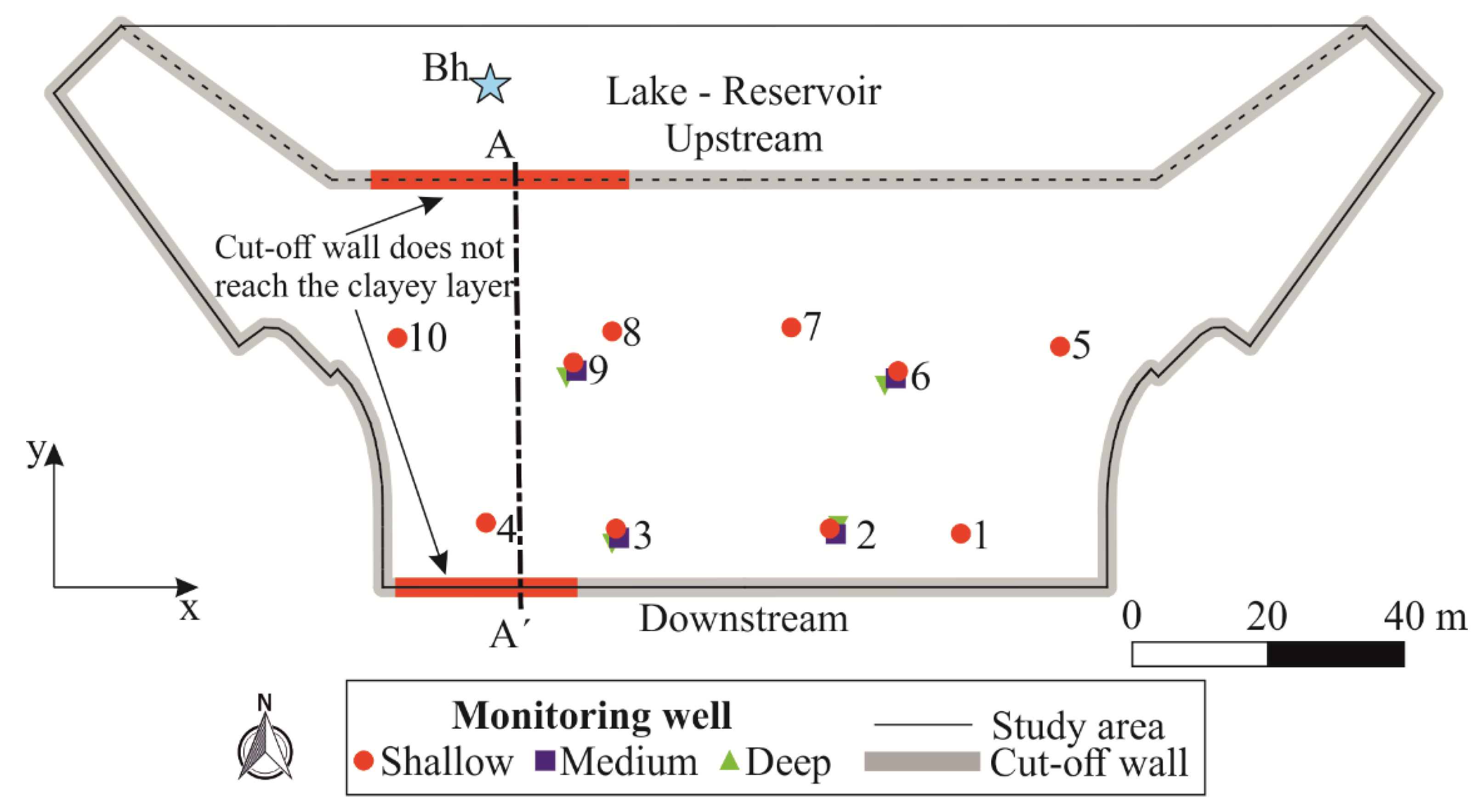
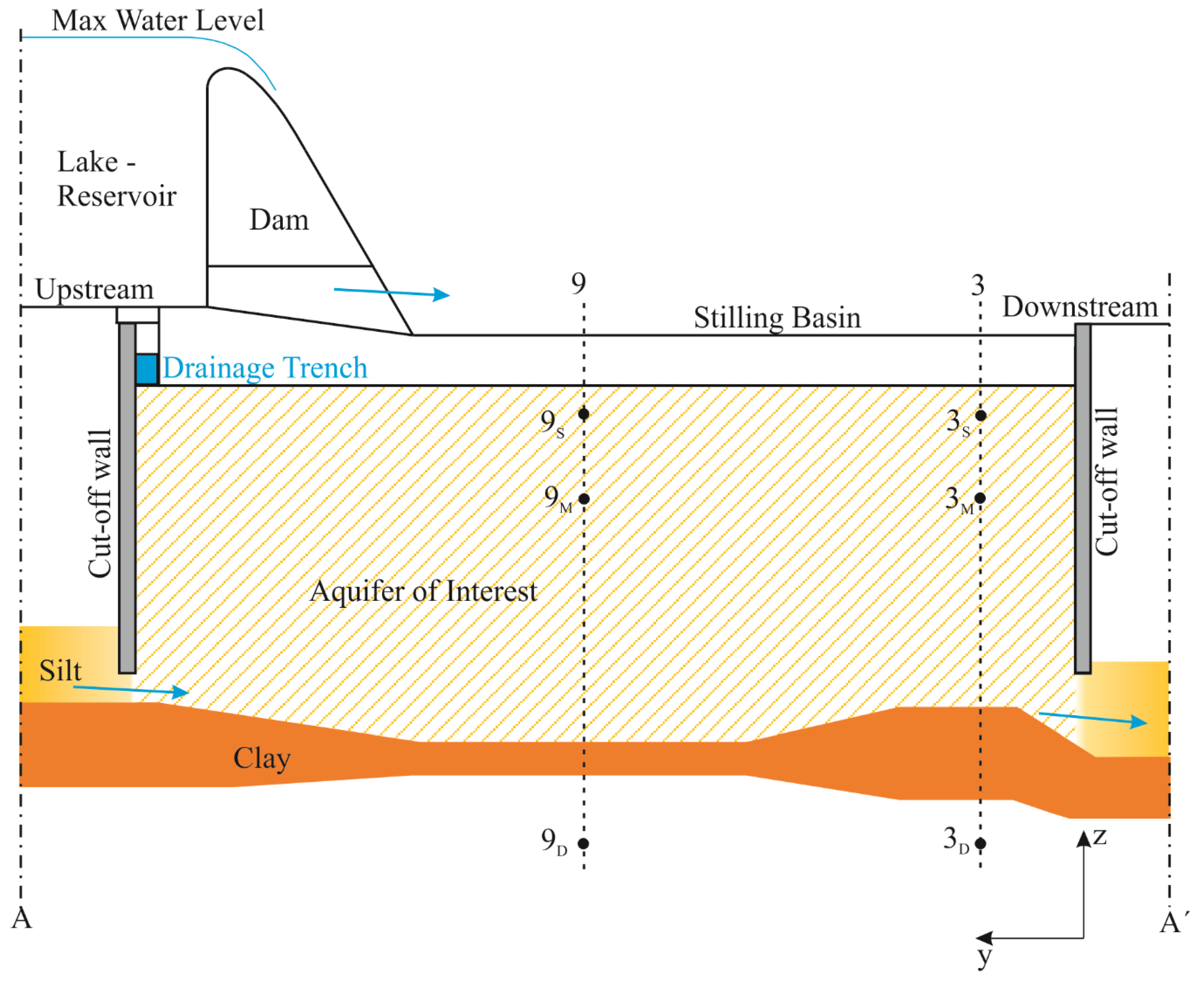
The case study is the aquifer underneath the main hydraulic structure (Figure 1 and Figure 2) of a flood control reservoir located in northern Italy. The structure is designed to dampen the river flood waves storing, in a reservoir, the excess water of high return period floods and releasing it downstream at a controlled rate. The main structure is a concrete dam (about 15 m high and 200 m long) placed at the downstream section of the reservoir (storage volume about 10 Mm³). A stilling basin, designed to dissipate the energy of the discharged flow, is located immediately downstream of the dam. The stilling basin bottom consists of concrete slabs, and dissipating blocks are located above them. The deposits below the dam and the stilling basin are surrounded by a cut-off wall (20–25 m deep) with the aim of obtaining an isolated “box” (Figure 1 and Figure 2). The box is designed to limit the interactions between the water in the reservoir and the aquifer underneath the dam and the basin; in particular, the objective of the wall is to prevent excessive uplift forces on the entire structure. The uplift force consists of an upward pressure at the interface between the structure and its permeable foundation [26], due to the increased hydraulic heads in the aquifer caused by the raising water levels in the lake. Because, on gravity dams, the uplift forces decrease the effective weight of the structure, they must be controlled and reduced to avoid stability problems. For this reason, in addition to the cut-off wall, the groundwater heads inside the box are also conditioned by a 110 m long drainage trench located upstream of the dam, about 3 m below its bottom (Figure 2).

The lithology of the study area can be well outlined by means of three layers: A phreatic aquifer (from 0 to 20 m depth) with prevailing silty gravels, a thin clayey layer (25 to 30 m) and a regional semi-confined aquifer (beneath 30 m). This system was investigated by means of different borehole logs obtained by drilling inside the box (four) and its surroundings (five) for a depth of about 35 m. Fourteen monitoring wells (Figure 1 and Figure 2) are within the studied area and they can be subdivided into three categories: Shallow (from 3 to 10 m, named S), medium (from 10 to 20 m, named M) and deep (from 30 to 40 m, named D).

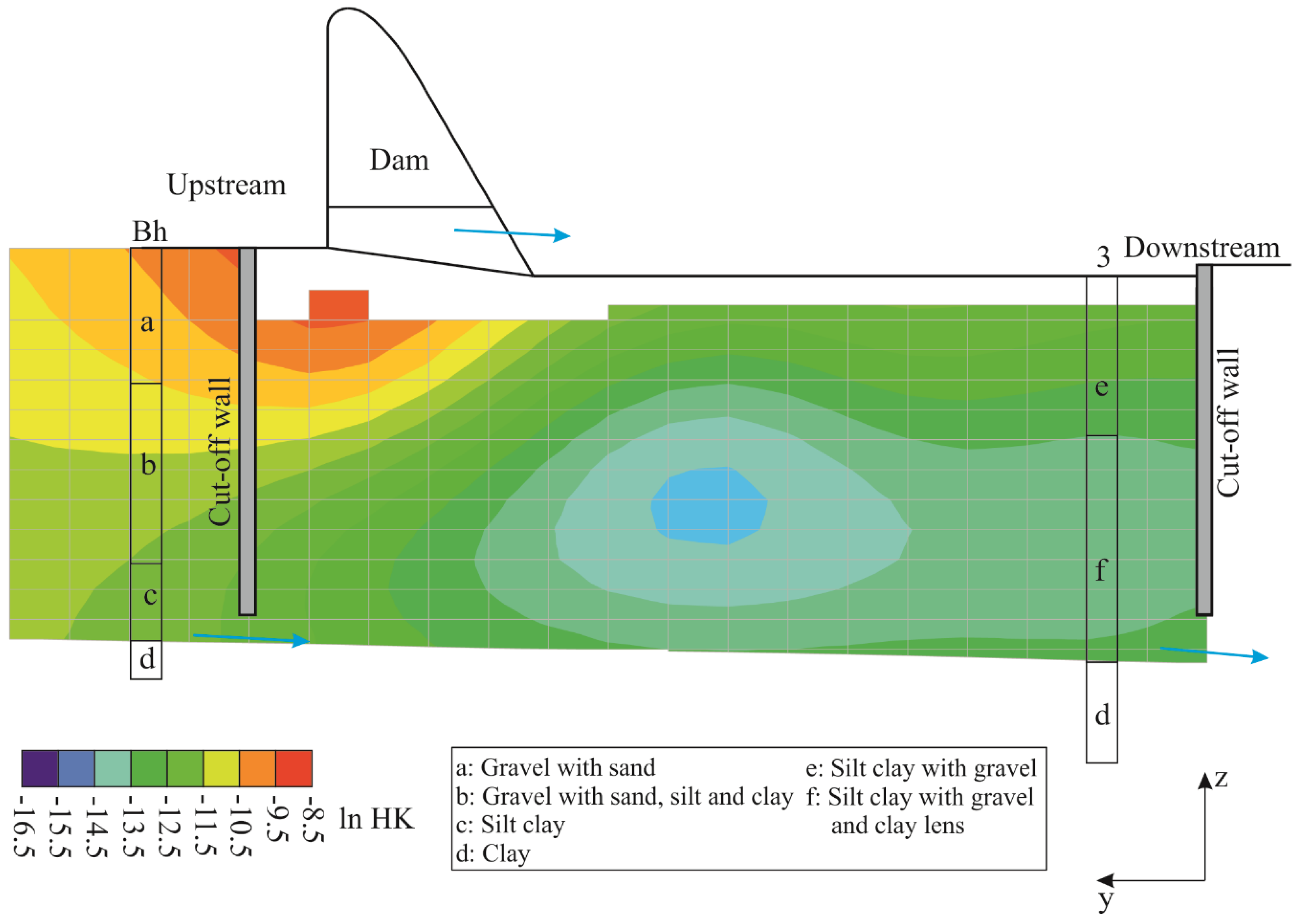
After the completion of the structure, different phases of investigation, control and monitoring of the efficiency of the entire system have been carried out to highlight the interactions between the reservoir and the aquifer beneath, in particular the one within the cut-off wall. During these tests (a period of about five months overall), the reservoir was filled and maintained at different stages up to the maximum level. Although the structure was completely safe throughout the entire investigation period, some of the water levels in the monitoring points within the cut-off wall were highly correlated to the reservoir water stage. For this reason, further investigations were planned: First of all, four boreholes were drilled in the area close to the cut-off wall. The analysis of the new borehole logs allowed us to identify with higher accuracy the depth of the wall and the clayey layer. The structure presents two different behaviors from east to west. In the eastern part of the structure, the cut-off wall reaches the clayey layer, whereas in the western part, both on the upstream and downstream sides, the wall extends to a low HK layer that is on the top of the main clayey layer. Figure 2 shows a sketch view of the cross-section AA’ depicted in Figure 1.

During the investigation phase, the water levels inside the monitoring wells underneath the stilling basin were recorded every 2 h, and the lake stage was stored every 15 min. All the data were automatically collected through pressure probes and posted on a webserver in order to allow remote access of the information. The collected data were used to calibrate, through inverse modeling, a numerical flow model of the aquifer within the cut-off wall and above the clayey layer with the aim of reproducing the effect of the lake on the system, providing a tool that allows the forecasting of groundwater levels inside the box under different conditions.

2.2. Inverse Approach

In this work, the BGA [13,27] is adopted to solve the inverse problem. The BGA allows the estimating of a set of parameters in the context of highly parameterized inversion problems (many more parameters than observations) where the unknowns are distributed in space and/or time, providing the best reproduction of the available observations. The inversion is also constrained by means of prior information about the structure of the unknowns making use of geostatistical autocorrelation functions. The BGA has been developed and mainly tested in spatial field estimation problems, e.g., references [10,28,29], but performs well also in the context of autocorrelated time functions [30,31,32,33,34]. In the following, only an introduction of the inverse methodology is provided; for more mathematical details see, for example, references [13,35,36].

According to the measurement equation, for a discrete problem, observations (data vector $y$ $[n_o\times 1]$, aquifer hydraulic heads in this case) and parameters (unknown vector $s$ $[n_p\times 1]$, HK values in this work) are related by the following equation:

$$y=h(s)+r,$$

(1)

where $h(s)$ represents the forward model and $r$ $[n_o\times 1]$ denotes the epistemic error or noise vector.

The Bayes theorem, in terms of random variables and their probability density function (pdf) for the multivariate case, states that the posterior pdf of the parameters for given data, $p(s|y)$, is proportional to the product of the prior pdf of the data $p(s)$ and the likelihood function $L(y|s)$:

$$p(s|y)\propto p(s)L(y|s).$$

(2)

The parameter vector $s$ is assumed multi-Gaussian with prior mean $E[\mathbf{s}]=\mathbf{X}\mathsf{\beta }$ and prior covariance matrix $E[(\mathbf{s}-\mathbf{X}\mathsf{\beta }){(\mathbf{s}-\mathbf{X}\mathsf{\beta })}^{\mathrm{T}}]=Q$, where $E$ means the expected value, $X$ $[n_p\times p]$ is a matrix of base functions and $\beta$ $[p\times 1]$ is a vector of drift coefficients. The matrix $X$ maps each parameter with the corresponding $\beta$ (which are unknowns and estimated together with $s$) and, if necessary, can express a trend in the prior mean. Different values of $\beta$ (and consequently of mean values) are used to introduce a correlation partitioning in the unknown field and/or to estimate parameters of different types. The likelihood function is also assumed multi-Gaussian and the epistemic uncertainties $r$ are represented as a random process with zero mean and covariance matrix $R$.

When a linear model relates the unknowns to the data, $h(s)$ can be substituted with $Hs$ where the matrix $H$ $[n_o{\times n}_p]$ is independent from $s$; with these assumptions the posterior pdf (multi-Gaussian) is:

$$p(s|y)\propto \underset{\mathrm{Prior}}{\underbrace{\exp \left(-\raisebox{1ex}{$1$}\!\left/ \!\raisebox{-1ex}{$2$}\right.{(s-\mathbf{X}\beta )}^{\mathrm{T}}{Q}^{-1}(s-\mathbf{X}\beta )\right)}} \underset{\mathrm{Likelihood}}{\underbrace{\exp \left(-\raisebox{1ex}{$1$}\!\left/ \!\raisebox{-1ex}{$2$}\right.{(y-Hs)}^{\mathrm{T}}{R}^{-1}(y-Hs)\right)}}$$

(3)

and the best estimates of $s$ and $\beta$ are the posterior values that maximize Equation (3) obtained solving a linear system of equations [35].

Nonlinear problems can be solved by successively linearizing the measurement equation using an iterative procedure (quasi-linear approach, [13]); at each iteration $k$ in the linearization process $h(s)\approx h(s_k)+\tilde{H}(s-s_k)$ where $\tilde{H}$ is the sensitivity matrix (Jacobian) that must be evaluated at each iteration:

$$\tilde{H}={\frac{\partial h}{\partial s}|}_{s=s_k}.$$

(4)

In this work, the Jacobian was evaluated using an adjoint state methodology where the number of runs of the forward model needed for the Jacobian evaluation is related to the number of observations rather than the number of the parameters, allowing to reduce the computational time. To avoid numerical instabilities due to the nonlinearities of the forward model, an optimization procedure, “line search” [37] was adopted to drive the inverse solution.

A parametric exponential covariance function [21] (with variance ${\sigma }_s^2$ and correlation length $l$) was adopted to a priori characterize the HK field; the epistemic errors were assumed independent and identically distributed with variance ${\sigma }_R^2$.

In the context of “empirical Bayes”, the parameters of the covariance function (also known as structural parameters or hyperparameters), can be estimated from the data. The right selection of the hyperparameters is crucial to reach a proper solution of the inverse problem; in this work, we adopted a Bayesian adaptation [21] of the Restricted Maximum Likelihood method of Kitanidis [13]. Due to the nonlinearity of the forward problem, parameters $s$ and structural parameters must be estimated iteratively [28]. At the end of the inverse process, the posterior covariance matrix of the parameters [35] can be used to evaluate the uncertainty of the unknowns.

The package bgaPEST [21], a free software that implements the BGA with the PEST [38] concepts, was used in this work for the inversion.

2.3. Flow Model and Calibration

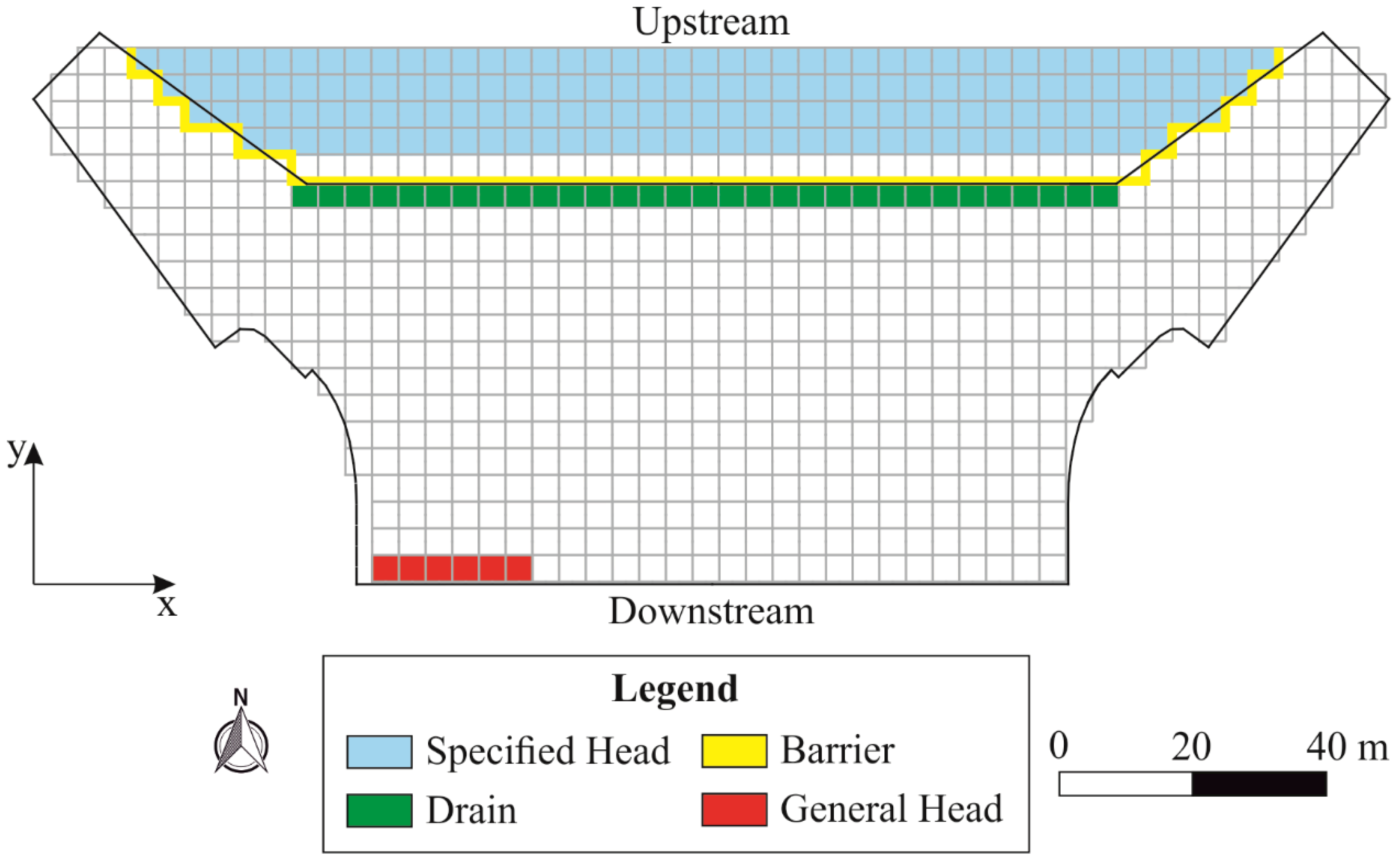
The flow processes in the aquifer underneath the structure and the stilling basin were investigated by means of a finite difference numerical model developed in MODFLOW 2005 [25]. The model has a grid of 20 rows, 50 columns and 13 layers (layer 1 is at the top of the model and layer 13 at the bottom) and covers an area of about 12,000 m². The cells are on a regular grid in the plane (4 m × 4 m) and are 2 m thick except for the top and bottom layers where they follow the structure and the clayey layer, respectively. The 13 layers are useful to reproduce, with accuracy of 2 m, the length of the cut-off wall (variable from 16 to 24 m from ground level) and to better describe the aquifer heterogeneity. The groundwater flow model extends for a small portion inside the reservoir, upstream of the cut-off wall, to take into account the interactions between the water in the lake and the aquifer below (Figure 3). According to the modeled area, the active cells are 8181. To adequately reproduce the conceptual model of the study domain (Figure 1), several types of boundary conditions (BCs) were considered. The lake, upstream of the dam, was represented by means of a specified head BC (layer 1), the drainage trench under the structure was modeled using the drain package of MODFLOW (layer 1), and the horizontal flow barrier (HFB) package (layers 1–12) was used to simulate the cut-off wall that delimits the box below the dam. The HFB package was developed [39] to simulate barriers to flow such as slurry and cut-off walls by reducing the conductance between pairs of adjacent cells in the finite difference grid. As an additional parameter, the HFB package requires a hydraulic characteristic that is the ratio between the hydraulic conductivity of the barrier and the thickness of the barrier. Considering that the cut-off wall consists of concrete 1 m thick, we assumed $5\times {10}^{-10} {\mathrm{s}}^{-1}$ as hydraulic characteristic value; for more details on how to compute heads close to hydraulic barrier, see also references [40,41]. The lateral and downstream boundary conditions were no flow except for the locations where the cut-off wall does not reach the clayey layer; this region was described by means of a general head BC (layers 9–13). Figure 3 shows the computational grid and summarizes the location of the boundary conditions. The top and bottom of the model were also considered impervious.

The model simulates, in unsteady state conditions, 145 days of the investigation period of the hydraulic structure during which the lake stage was step-by-step modified. Given that the initial condition of the groundwater model (in terms of hydraulic heads) was considered as the result of a preliminary steady state run, with the aim of avoiding influences from the starting values, the first 25 days of the simulation were treated as a warm-up period. The upstream specified head BC was based on the recorded lake stages with a temporal discretization of one day; the outlet of the groundwater model (general head BC) was related to the hydraulic heads observed downstream of the box in proximity of the involved region. The drain parameters were based on its geometry and the characteristics of the material used during the construction of the dam.

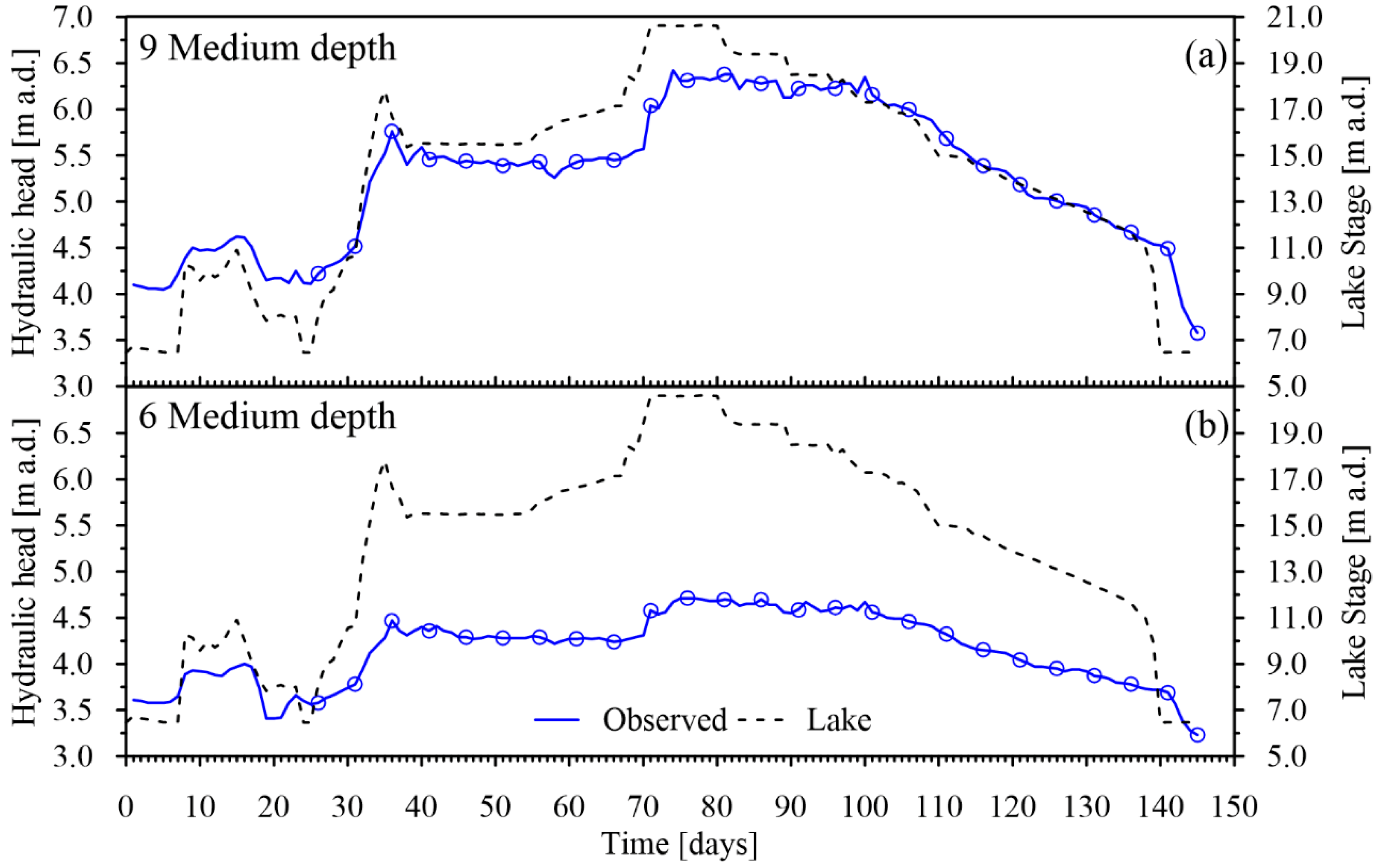
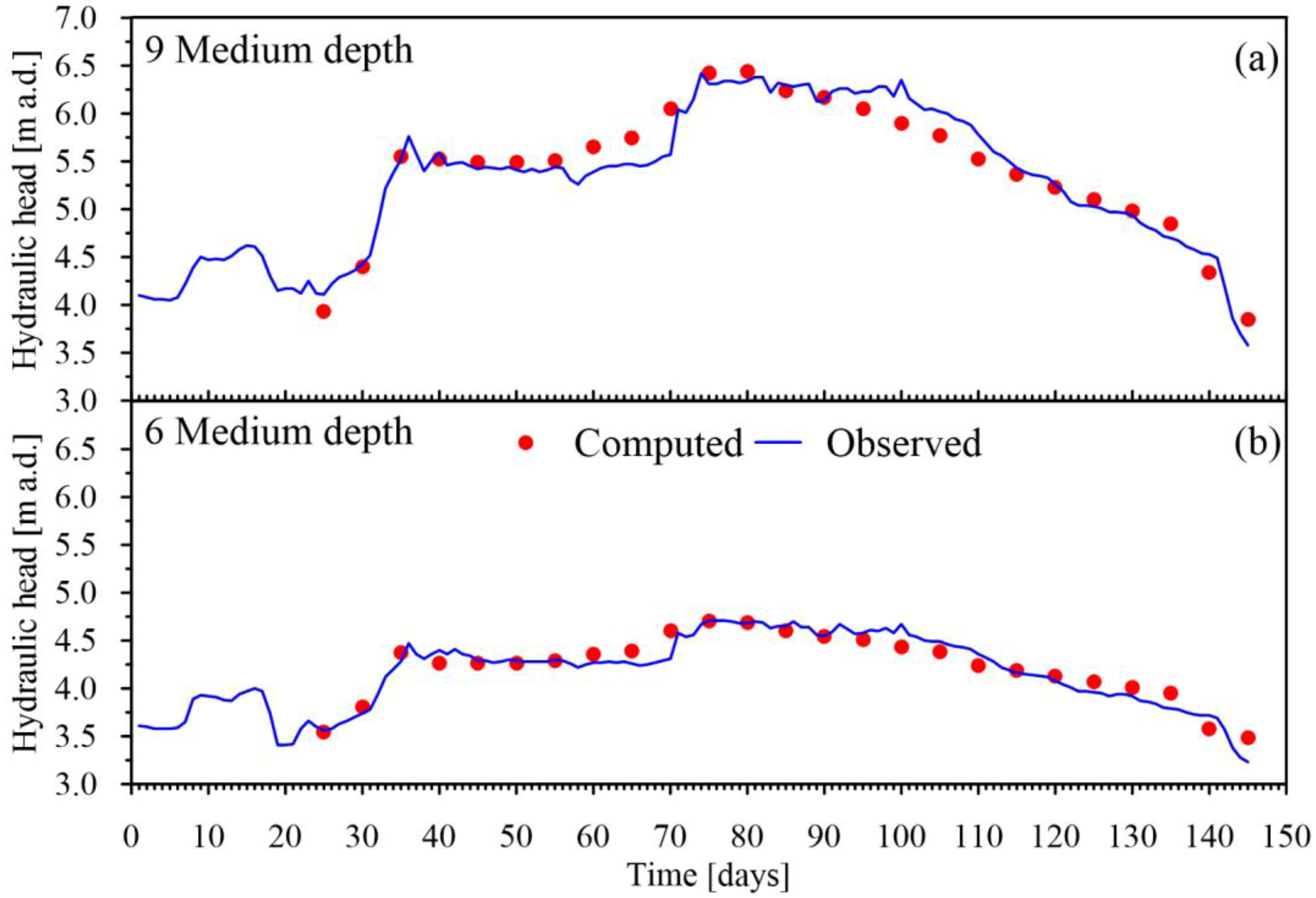
In addition to the boundary conditions, appropriate hydraulic parameters must be specified for the groundwater model; in particular, the HK and the specific storage are needed for each active cell. These parameters must be calibrated to closely reproduce the behavior of the real aquifer system; for this purpose, in this work, we used the observed head data in the monitoring wells. In particular, the data collected in 14 observation locations (locations 1 to 10 at shallow depth and locations 2, 3, 6 and 9 at medium depth, Figure 1 and Figure 2) were taken into account; for each monitoring point, we considered 25 observations over time (one every 5 days starting from day 26). The number of observations for each monitoring point is a compromise between the reasonable reproduction of the observed time-series and the computational time needed to perform the inversion. Figure 4a,b show, by way of example, the observed hydraulic head, respectively, at the monitoring wells 9M and 6M (see Figure 1 for the location); the same Figure 4 shows the lake stage observed upstream of the hydraulic structure for the studied period.

We performed a preliminary calibration of the hydraulic parameters using PEST [38] and a lumped approach, in which different zones (kept homogeneous) were identified according to the analysis of the borehole logs. This process aimed to find initial values for all the parameters. Then we used the Bayesian Geostatistical Approach to estimate the HK values for each of the 8181 active cells of the groundwater model; in the context of a highly parameterized inversion, each cell is an estimable parameter. The other hydraulic properties were equal to the values identified with the preliminary calibration. The HK field was estimated in a logarithmic space.

We adopted an adjoint-state formulation of MODFLOW 2005 [42] to calculate the sensitivities of each observation to each estimable parameter (Jacobian) required by the inverse approach. To speed up the computation we followed the recommendations of D’Oria et al. [43].

To evaluate the results of the inverse procedure, several performance metrics based on the observed and computed hydraulic heads ($H_{obs}$ and $H_{comp}$, respectively) were adopted: The mean error $\mathrm{ME}=H_{obs}-H_{comp}$, the mean absolute error $\mathrm{MAE}=|H_{obs}-H_{comp}|$, the root mean square error $\mathrm{RMSE}=\sqrt{{(H_{obs}-H_{comp})}^2/N}$ and the normalized root mean square error $\mathrm{nRMSE}=\left(\sqrt{{(H_{obs}-H_{comp})}^2/N}\right)/\Delta$; where $N$ is the number of observations and $\Delta$ represents the difference between the maximum and minimum observed hydraulic heads.

3. Results

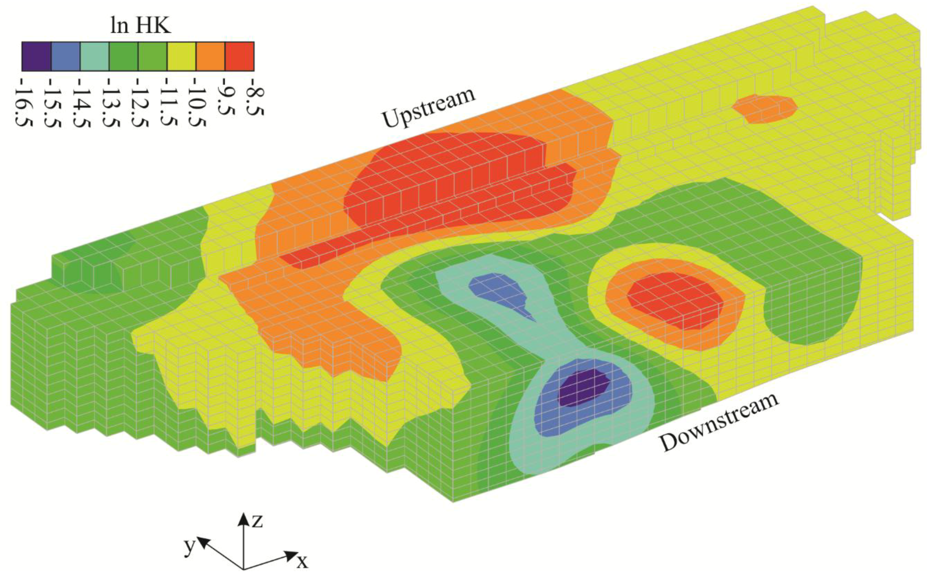
The estimation of the hydraulic conductivities (8181 HK values) based on the BGA and the groundwater head observations (350 data) is reported in Figure 5. The resulting HK field has a mean value equal to 1.8 × 10⁻⁵ m/s; in natural logarithmic scale the mean is −11.7 and the variance is 2.1.

The results indicate a moderate degree of heterogeneity of the estimated field, consistent with the alluvial nature of the aquifer and the analysis of the borehole logs. According to Figure 5, the area with the lowest HK values is close to the general head boundary conditions (see Figure 3).

Figure 6 shows, as example, the HK field of layer 10. The cyan-blue area identifies the lowest HK values, and the red area refers to the highest ones. Figure 7 depicts the HK field estimated at the vertical cross section AA’ of Figure 1 and, superimposed, the logs for borehole Bh and monitoring well 3 (the closest available to cross section AA’). Borehole Bh can be simplified in four groups of soil types starting from the ground level: Gravel with sand, gravel with sand and silt, silt clay, and clay. Monitoring well 3 can be described with three soil types starting from the ground level: Silt clay with gravel, silt clay with gravel and clay lenses, and clay. The clay material in both boreholes indicates the impervious bottom of the studied aquifer. The analysis of Figure 6 and Figure 7 confirms that a zone with low conductivities is located close to the outlet of the box, and this is consistent with the outcomes of the borehole logs.

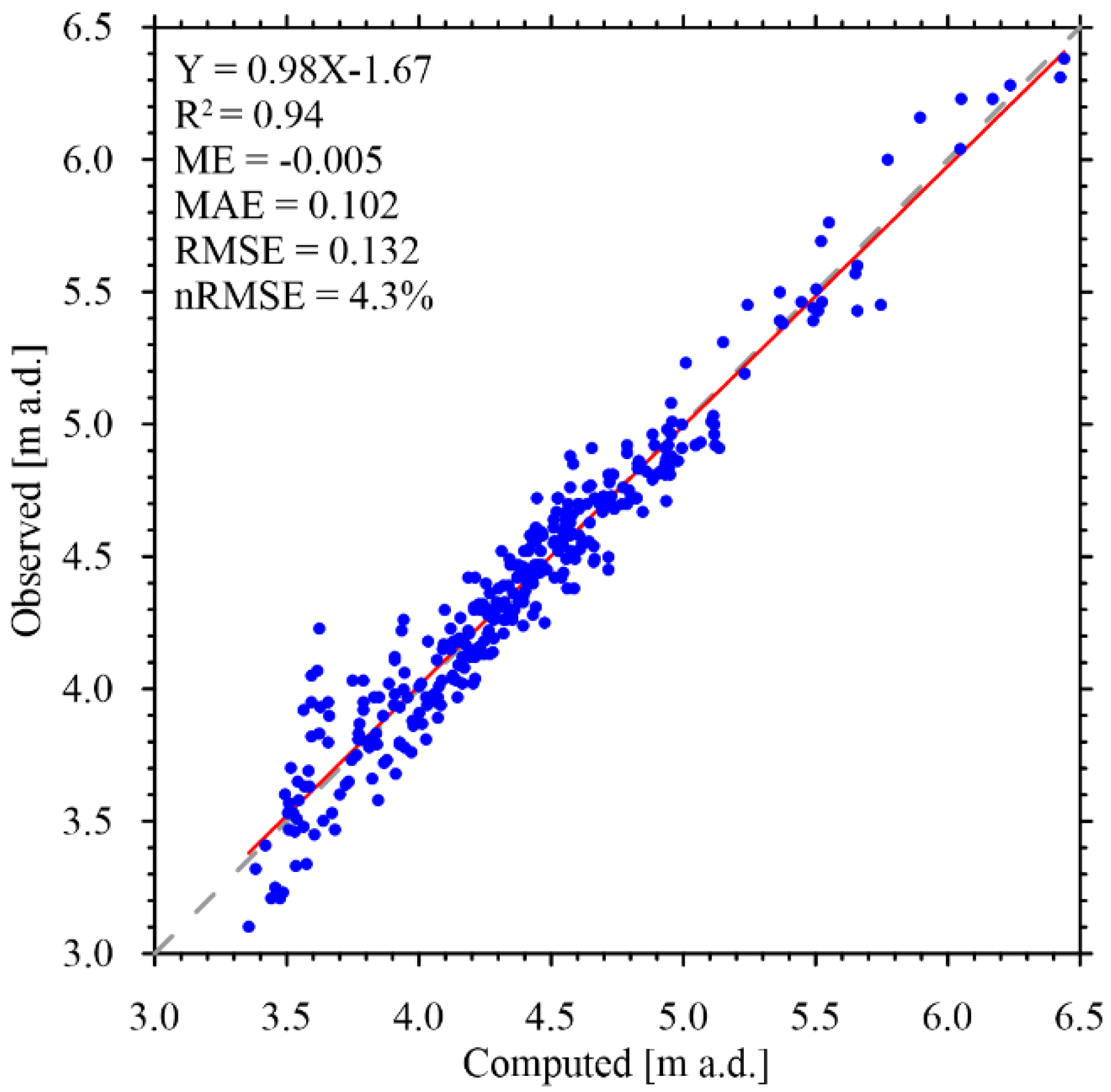
In applying the inverse procedure, the epistemic error variance, ${\sigma }_R^2$, was set to $5\times {10}^{-3} {\mathrm{m}}^2$, a reasonable level of uncertainty for the hydraulic heads to be reproduced by means of BGA. Figure 8 reports the observed values versus the modeled ones for all the 350 records together with their best linear fit and the coefficient of determination. A good agreement between the observed and modeled hydraulic heads exists overall and no over-fitting problems seem to arise in the estimation. The results have been evaluated analyzing the performance metrics described above and shown in Figure 8; according to reference [44], the obtained values confirm the quality of the inverse procedure.

Figure 9a,b show, as example, the observed and computed hydraulic heads at the monitoring wells 6 M and 9 M. The calibrated numerical model is able to properly reproduce the hydraulic heads, at the monitoring wells, related to the lake stage variations.

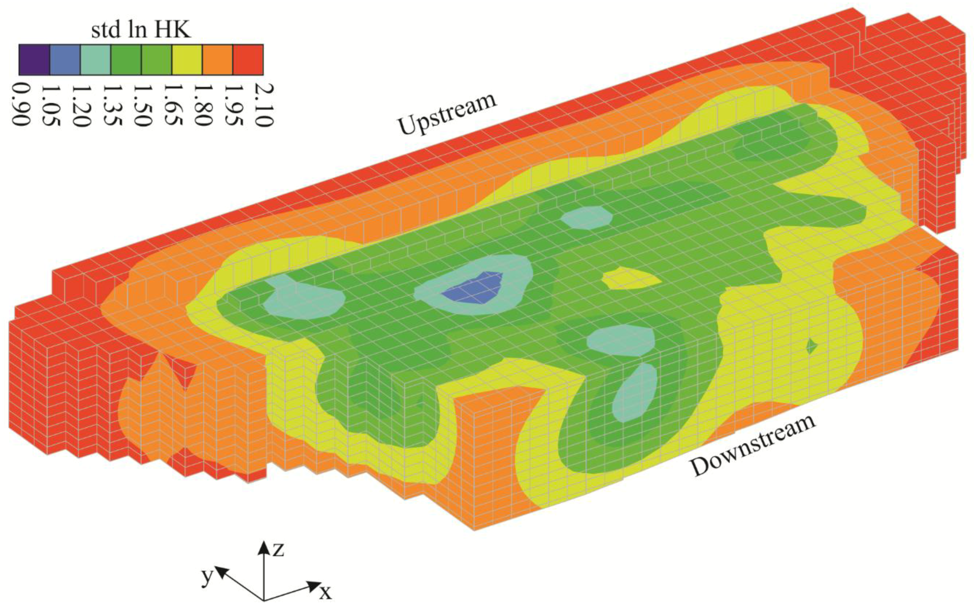
The BGA allows us also to compute the uncertainty of the estimates from the posterior covariance matrix. Figure 10 reports the logarithm of the standard deviation of the estimated HK field. As expected, in Figure 8, the smaller standard deviation values are in the area between the monitoring wells where more information is available thanks to the natural stimuli of the aquifer. The mean value of the posterior standard deviation is 1.7.

The parameters of the exponential covariance function that a priori characterizes the HK field, variance ${\sigma }_s^2$ and correlation length $l$, estimated by bgaPEST during the inverse procedure are equal to 4.4 (natural logarithmic scale) and 17.9 m, respectively.

4. Discussion and Conclusions

In this work, we estimated the HK field of a portion of the aquifer underneath a flood protection structure. The study is useful to understand and evaluate the interactions between the lake upstream of the dam and the groundwater levels that could cause stability problems to the structure due to excessive uplift forces. In the past, the structure and the surrounding aquifer have been deeply investigated through monitoring wells, boreholes and geological surveys. These investigations allowed us to develop at first a very accurate conceptual model and then a numerical groundwater flow model. Unfortunately, the HK of the investigated aquifer was not known. To solve this problem, we made use of a well-known BGA that simultaneously allows one to estimate the unknown parameters (HK at grid cells) and the structural parameters of the selected covariance model.

A common issue in aquifer parameter estimation is the lack of observations. To overcome this problem, in this work, we considered the hydraulic heads, observed at the monitoring wells, related to the variations of the lake stage (natural stimuli) upstream of the structure.

The BGA was able to estimate a large number of unknowns (8181 grid nodes) using the hydraulic head information collected at 14 monitoring points at 25 different times. A moderate degree of heterogeneity is estimated for the HK field during the inversion of the hydraulic heads. The results are consistent with the alluvial nature of the investigated aquifer, the evidence of the borehole logs and the information content of the data. The BGA, together with the estimation of the hyperparameters using the Bayesian adaptation of the Restricted Maximum Likelihood method, provides the smoothest solution consistent with the observations; however, a certain degree of complexity can be found in the results since it is supported by the available data. The hydraulic heads computed considering the estimated HK field were very close to the observed one. In fact, the mean absolute error is close to 10 cm and the normalized root mean square error is very small (4.3%) considering the complexity of the study case.

The calibrated groundwater model allowed us to better understand the interactions between the reservoir and the studied aquifer under different scenarios and to forecast the hydraulic head levels in the investigated “box” due to strong flood events.

The use of natural stimuli to estimate the hydraulic heterogeneity of aquifers seems promising in those situations where traditional techniques, such as pumping tests, are not feasible for budget or practical problems.

References

- Petit-Boix, A.; Sevigné-Itoiz, E.; Rojas-Gutierrez, L.A.; Barbassa, A.P.; Josa, A.; Rieradevall, J.; Gabarrell, X. Floods and consequential life cycle assessment: Integrating flood damage into the environmental assessment of stormwater Best Management Practices. J. Clean. Prod. 2017, 162, 601–608. [Google Scholar] [CrossRef]
- Lyu, H.-M.; Sun, W.-J.; Shen, S.-L.; Arulrajah, A. Flood risk assessment in metro systems of mega-cities using a GIS-based modeling approach. Sci. Total Environ. 2018, 626, 1012–1025. [Google Scholar] [CrossRef]
- Lyu, H.-M.; Shen, S.-L.; Zhou, A.; Yang, J. Perspectives for flood risk assessment and management for mega-city metro system. Tunn. Undergr. Space Technol. 2019, 84, 31–44. [Google Scholar] [CrossRef]
- Berg, S.J.; Illman, W.A. Comparison of Hydraulic Tomography with Traditional Methods at a Highly Heterogeneous Site. Groundwater 2015, 53, 71–89. [Google Scholar] [CrossRef] [PubMed]
- Xu, T.; Gómez-Hernández, J.J. Simultaneous identification of a contaminant source and hydraulic conductivity via the restart normal-score ensemble Kalman filter. Adv. Water Resour. 2018, 112, 106–123. [Google Scholar] [CrossRef]
- Xu, T.; Gómez-Hernández, J.J. Inverse sequential simulation: A new approach for the characterization of hydraulic conductivities demonstrated on a non-Gaussian field. Water Resour. Res. 2015, 51, 2227–2242. [Google Scholar] [CrossRef] [Green Version]
- Marinoni, M.; Delay, F.; Ackerer, P.; Riva, M.; Guadagnini, A. Identification of groundwater flow parameters using reciprocal data from hydraulic interference tests. J. Hydrol. 2016, 539, 88–101. [Google Scholar] [CrossRef]
- Zanini, A.; Tanda, M.G.; Woodbury, A.D. Identification of transmissivity fields using a Bayesian strategy and perturbative approach. Adv. Water Resour. 2017, 108, 69–82. [Google Scholar] [CrossRef]
- Butera, I.; Soffia, C. Cokriging transmissivity, head and trajectory data for transmissivity and solute path estimation. Groundwater 2017, 55, 362–374. [Google Scholar] [CrossRef]
- D’Oria, M.; Zanini, A.; Cupola, F. Oscillatory pumping test to estimate aquifer hydraulic parameters in a Bayesian geostatistical framework. Math. Geosci. 2018, 50, 169–186. [Google Scholar] [CrossRef]
- Chen, Z.; Gómez-Hernández, J.J.; Xu, T.; Zanini, A. Joint identification of contaminant source and aquifer geometry in a sandbox experiment with the restart ensemble Kalman filter. J. Hydrol. 2018, 564, 1074–1084. [Google Scholar] [CrossRef]
- Comunian, A.; Giudici, M. Hybrid inversion method to estimate hydraulic transmissivity by combining multiple-point statistics and a direct inversion method. Math. Geosci. 2018, 50, 147–167. [Google Scholar] [CrossRef]
- Kitanidis, P.K. Quasi-linear geostatistical theory for inversing. Water Resour. Res. 1995, 31, 2411–2419. [Google Scholar] [CrossRef]
- Fienen, M.N.; Clemo, T.; Kitanidis, P.K. An interactive Bayesian geostatistical inverse protocol for hydraulic tomography. Water Resour. Res. 2008, 44. [Google Scholar] [CrossRef] [Green Version]
- D’Oria, M.; Lanubile, R.; Zanini, A. Bayesian estimation of a highly parameterized hydraulic conductivity field: A study case. Procedia Environ. Sci. 2015, 25, 82–89. [Google Scholar] [CrossRef]
- Kitanidis, P.K.; Lee, J. Principal component geostatistical approach for large-dimensional inverse problems. Water Resour. Res. 2014, 50, 5428–5443. [Google Scholar] [CrossRef]
- D’Oria, M.; Tanda, M.G. Reverse flow routing in open channels: A Bayesian geostatistical approach. J. Hydrol. 2012, 460–461, 130–135. [Google Scholar] [CrossRef]
- Ferrari, A.; D’Oria, M.; Vacondio, R.; Dal Palù, A.; Mignosa, P.; Tanda, M.G. Discharge hydrograph estimation at upstream-ungauged sections by coupling a Bayesian methodology and a 2-D GPU shallow water model. Hydrol. Earth Syst. Sci. 2018, 22, 5299–5316. [Google Scholar] [CrossRef]
- D’Oria, M.; Mignosa, P.; Tanda, M.G. An inverse method to estimate the flow through a levee breach. Adv. Water Resour. 2015, 82, 166–175. [Google Scholar] [CrossRef]
- Leonhardt, G.; D’Oria, M.; Kleidorfer, M.; Rauch, W. Estimating inflow to a combined sewer overflow structure with storage tank in real time: Evaluation of different approaches. Water Sci. Technol. 2014, 70, 1143–1151. [Google Scholar] [CrossRef]
- Fienen, M.N.; D’Oria, M.; Doherty, J.E.; Hunt, R.J. Approaches in Highly Parameterized Inversion: bgaPEST, a Bayesian Geostatistical Approach Implementation with PEST—Documentation and Instructions; U.S. Geological Survey: Reston, VA, USA, 2013; Volume 7.
- Yeh, T.-C.J.; Xiang, J.; Suribhatla, R.M.; Hsu, K.-C.; Lee, C.-H.; Wen, J.-C. River stage tomography: A new approach for characterizing groundwater basins. Water Resour. Res. 2009, 45. [Google Scholar] [CrossRef] [Green Version]
- Wang, Y.-L.; Yeh, T.-C.J.; Wen, J.-C.; Huang, S.-Y.; Zha, Y.; Tsai, J.-P.; Hao, Y.; Liang, Y. Characterizing subsurface hydraulic heterogeneity of alluvial fan using riverstage fluctuations. J. Hydrol. 2017, 547, 650–663. [Google Scholar] [CrossRef]
- Jardani, A.; Dupont, J.P.; Revil, A.; Massei, N.; Fournier, M.; Laignel, B. Geostatistical inverse modeling of the transmissivity field of a heterogeneous alluvial aquifer under tidal influence. J. Hydrol. 2012, 472–473, 287–300. [Google Scholar] [CrossRef]
- Harbaugh, A.W. MODFLOW-2005, the U.S. Geological Survey Modular Ground-Water Model—The Ground-Water Flow Process; U.S. Geological Survey Techniques and Methods: 6-A16; U.S. Geological Survey: Reston, VA, USA, 2005.
- Grishin, M.M. Hydraulic Structure; Mir Publishers: Moscow, Russia, 1982; Volume 1. [Google Scholar]
- Hoeksema, R.J.; Kitanidis, P.K. An Application of the Geostatistical approach to the inverse problem in two-dimensional groundwater modeling. Water Resour. Res. 1984, 20, 1003–1020. [Google Scholar] [CrossRef]
- Fienen, M.; Hunt, R.; Krabbenhoft, D.; Clemo, T. Obtaining parsimonious hydraulic conductivity fields using head and transport observations: A Bayesian geostatistical parameter estimation approach. Water Resour. Res. 2009, 45, W08405. [Google Scholar] [CrossRef]
- Cardiff, M.; Barrash, W.; Kitanidis, P.K. Hydraulic conductivity imaging from 3-D transient hydraulic tomography at several pumping/observation densities. Water Resour. Res. 2013, 49, 7311–7326. [Google Scholar] [CrossRef] [Green Version]
- Snodgrass, M.F.; Kitanidis, P.K. A geostatistical approach to contaminant source identification. Water Resour. Res. 1997, 33, 537–546. [Google Scholar] [CrossRef] [Green Version]
- Butera, I.; Tanda, M.G. A geostatistical approach to recover the release history of groundwater pollutants. Water Resour Res. 2003, 39, 1372. [Google Scholar] [CrossRef]
- Butera, I.; Tanda, M.G.; Zanini, A. Use of numerical modelling to identify the transfer function and application to the geostatistical procedure in the solution of inverse problems in groundwater. J. Inverse Ill-Posed Probl. 2006, 14, 547–572. [Google Scholar] [CrossRef]
- D’Oria, M.; Mignosa, P.; Tanda, M.G. Bayesian estimation of inflow hydrographs in ungauged sites of multiple reach systems. Adv. Water Resour. 2014, 63, 143–151. [Google Scholar] [CrossRef]
- Cupola, F.; Tanda, M.G.; Zanini, A. Laboratory sandbox validation of pollutant source location methods. Stoch. Environ. Res. Risk Assess. 2015, 29, 169–182. [Google Scholar] [CrossRef]
- Nowak, W.; Cirpka, O.A. A modified Levenberg–Marquardt algorithm for quasi-linear geostatistical inversing. Adv. Water Resour. 2004, 27, 737–750. [Google Scholar] [CrossRef]
- D’Oria, M.; Mignosa, P.; Tanda, M.G. Reverse level pool routing: Comparison between a deterministic and a stochastic approach. J. Hydrol. 2012, 470–471, 28–35. [Google Scholar] [CrossRef]
- Zanini, A.; Kitanidis, P.K. Geostatistical inversing for large-contrast transmissivity fields. Stoch. Environ. Res. Risk Assess. 2009, 23, 565–577. [Google Scholar] [CrossRef]
- Doherty, J. PEST, Model-Independent Parameter Estimation—User Manual. 5th Edition, with Slight Additions; Watermark Numerical Computing: Brisbane, Australia, 2010. [Google Scholar]
- Hsieh, P.A.; Freckleton, J.R. Documentation of a Computer Program to Simulate Horizontal-Flow Barriers Using the U.S. Geological Survey’s Modular Three-Dimensional Finite-Difference Ground-Water Flow Model; U.S. Geological Survey: Reston, VA, USA, 1993.
- Shen, S.-L.; Wu, Y.-X.; Misra, A. Calculation of head difference at two sides of a cut-off barrier during excavation dewatering. Comput. Geotech. 2017, 91, 192–202. [Google Scholar] [CrossRef]
- Wu, Y.-X.; Shen, S.-L.; Yuan, D.-J. Characteristics of dewatering induced drawdown curve under blocking effect of retaining wall in aquifer. J. Hydrol. 2016, 539, 554–566. [Google Scholar] [CrossRef]
- Clemo, T. MODFLOW-2005 Ground Water Model—User Guide to the Adjoint State Based Sensitivity Process (ADJ); Center for the Geophysical Investigation of the Shallow Subsurface Boise State University: Boise, ID, USA, 2007. [Google Scholar]
- D’Oria, M.; Fienen, M.N. MODFLOW-Style parameters in underdetermined parameter estimation. Ground Water 2012, 50, 149–153. [Google Scholar] [CrossRef]
- Anderson, M.P.; Woessner, W.W. Applied Groundwater Modeling: Simulation of Flow and Advective Transport; Academic Press: San Diego, CA, USA, 1992; ISBN 0-12-059485-4. [Google Scholar]
Figure 1.
Top view of the study area: Location of the monitoring wells and of the cross-section AA’ of Figure 2. The cyan star denotes the position of the borehole Bh.
Figure 2.
Sketch view of the vertical cross section (AA’) of the investigated area with the indication of the aquifer of interest. Figure not to scale. Monitoring wells no. 9 and no. 3 with the indication of the observation depth: Shallow (S), medium (M) and deep (D). The plan view is shown in Figure 1.
Figure 3.
Model grid and types of boundary conditions. The black line is the external boundary of the dam and the stilling basin; the gray lines represent the computational grid used to model the study area.
Figure 4.
Lake stage above datum (a.d.) during the analyzed 145 days (a,b), observed hydraulic heads in two monitoring wells: no. 9 (a) and no. 6 (b), both at medium depth. The circles identify the hydraulic heads used in the inversion process. The location of the monitoring points is reported in Figure 1.
Figure 5.
Three-dimensional view of the estimated hydraulic conductivity field: The results are reported in terms of natural logarithm of the parameters (ln HK) with units m/s in the physical space.
Figure 6.
Estimated hydraulic conductivity field for layer 10: The results are reported in terms of natural logarithm of the parameters (ln HK) with units m/s in the physical space.
Figure 7.
Estimated hydraulic conductivity field for Section AA’ of Figure 1: The results are reported in terms of natural logarithm of the parameters (ln HK) with units m/s in the physical space. Logs for borehole Bh and monitoring well 3 (see Figure 1).
Figure 8.
Observed versus computed hydraulic heads (350 data), best linear fit (solid line, with equation) and its coefficient of determination R2 and performance metrics: Mean error ME, mean absolute error MAE, root mean square error RMSE and normalized one nRMSE. The 45-degrees line (dashed line) is reported for comparison.
Figure 9.
Observed and computed hydraulic heads above datum (a.d.) during the analyzed 145 days in two monitoring wells: (a) no. 9 (b) no. 6, both at medium depth. The location of the monitoring points is reported in Figure 2.
Figure 10.
Three-dimensional view of the standard deviation (SD) of the estimated hydraulic conductivity field. The results are reported in terms of natural logarithm of the parameters (ln HK) with units m/s in the physical space.
© 2019 by the authors. Licensee MDPI, Basel, Switzerland. This article is an open access article distributed under the terms and conditions of the Creative Commons Attribution (CC BY) license (http://creativecommons.org/licenses/by/4.0/).
Share and Cite
MDPI and ACS Style
D’Oria, M.; Zanini, A. Characterization of Hydraulic Heterogeneity of Alluvial Aquifer Using Natural Stimuli: A Field Experience of Northern Italy. Water 2019, 11, 176. https://doi.org/10.3390/w11010176
AMA Style
D’Oria M, Zanini A. Characterization of Hydraulic Heterogeneity of Alluvial Aquifer Using Natural Stimuli: A Field Experience of Northern Italy. Water. 2019; 11(1):176. https://doi.org/10.3390/w11010176
Chicago/Turabian StyleD’Oria, Marco, and Andrea Zanini. 2019. "Characterization of Hydraulic Heterogeneity of Alluvial Aquifer Using Natural Stimuli: A Field Experience of Northern Italy" Water 11, no. 1: 176. https://doi.org/10.3390/w11010176
Note that from the first issue of 2016, this journal uses article numbers instead of page numbers. See further details here.