A Novel ArcGIS Toolbox for Estimating Crop Water Demands by Integrating the Dual Crop Coefficient Approach with Multi-Satellite Imagery

Abstract

Advances in information and communication technologies facilitate the application of complex models for optimizing agricultural water management. This paper presents an easy-to-use tool for determining crop water demands using the dual crop coefficient approach and remote sensing imagery. The model was developed using Python as a programming language and integrated into an ArcGIS (geographic information system) toolbox. Inputs consist of images from satellites Landsat 7 and 8, and Sentinel 2A, along with data for defining crop, weather, soil type, and irrigation system. The tool produces a spatial distribution map of the crop evapotranspiration estimates, assuming no water stress, which allows quantifying the water demand and its variability within an agricultural field with a spatial resolution of either 10 m (for Sentinel) or 30 m (for Landsat). The model was validated by comparing the estimated basal crop coefficients (K_cb) of lettuce and peach during an irrigation season with those tabulated as a reference for these crops. Good agreements between K_cb derived from both methods were obtained with a root mean squared error ranging from 0.01 to 0.02 for both crops, although certain underestimations were observed resulting from the uneven crop development in the field (percent bias of −4.74% and −1.80% for lettuce and peach, respectively). The developed tool can be incorporated into commercial decision support systems for irrigation scheduling and other applications that account for the water balance in agro-ecosystems. This tool is freely available upon request to the corresponding author.

1. Introduction

The important technological advances that have taken place in recent years allow for obtaining a greater predictive capacity and a more accurate assessment of different processes within agricultural systems [1]. These advances have enabled the generation of models for the estimation of plant chemical and biophysical parameters for improving pest and disease management [2,3], nutrient assessment [4,5], irrigation scheduling [6,7], and yield predictions [8,9]. Nevertheless, they frequently result in models that are difficult to apply to generate real solutions for the agricultural sector, as a consequence of limitations in public access to data, privacy and confidentiality issues, lack of funding for long-term collection and curation of data, and technical difficulties in managing and sharing data [10].

For the specific case of crop evapotranspiration (ET_c) estimation, several models have been developed following different approaches; the most common among them are those based on surface energy balance (SEB) and soil water balance (SWB). Most of these models are too complex for non-specialized users, as in the case of many farmers, and even by more qualified users such as technicians from irrigation communities or agricultural cooperatives. This low level of practical applicability is caused by the fact that these models are usually composed of a large number of variables and parameters, requiring, in many cases, long execution times [11,12]. In addition, ET_c is usually computed on a punctual location that may not be representative of the entire irrigated area. Using remote sensing technologies appears to be an efficient and economic approach to provide evapotranspiration (ET) estimations on large areas, allowing the assessment of the ET spatial variability [13].

The most common methodologies for ET estimation from remotely sensed imagery are those based on SEB and those based on vegetation indexes (VI). Models based on SEB take advantage of the relationship between surface reflectance data and energy balance components to derive ET_c. Latent heat flux, and thus ET, is computed as the residual component of the SEB at the time of satellite overpass by subtracting the soil heat flux and sensible heat flux from the net radiation at the surface. In all SEB models, surface temperature data play a critical role in the estimation of crop water requirements. Nevertheless, spatial resolution improvements of satellites have occurred mainly in the visible and near infrared (VNIR) regions, whereas the thermal domain has remained at the same (or even lower) spatial resolution as that provided in the early 1980s [14]. Thus, the resulting pixel size limits the use of SEB models, especially for heterogeneous crops. In addition, SEB approaches need to extrapolate the instantaneous ET (ET_inst) obtained at the time of the satellite pass to daily values, which can be usually done by assuming the conservation of the evaporative fraction or the ratio of ET to reference evapotranspiration, ET_o [15,16]. A recent study in Mexico showed that using the MOD16 algorithm for ET estimation, through an SEB model, on wheat crops and shrub lands had an average underestimation of 0.32 mm·day⁻¹ (up to 1.48 mm·day⁻¹ in certain cases) with respect to ET measurements in the field using eddy covariance equipment [17].

An alternative to SEB models is using VI-based approaches, which compute ET from empirical, site-specific relationships between the fraction of ground covered by vegetation and VI (for example, the normalized difference vegetation index (NDVI) or the soil-adjusted vegetation index (SAVI)). However, VI reflect the vegetation cover conditions of a given date for estimating the actual basal crop coefficient (K_cb), but require an additional approach, normally a water balance model, to estimate the evaporation coefficient (K_e). In addition, most VI-based methods assume baseline conditions (e.g., no soil water limitations) as being unable to consider the impact of soil water shortage, salinity, or disease on the estimation of the crop coefficient (K_c) [7,18]. In this sense, previous reports indicated that, despite some drawbacks and an average error of 0.75 mm·day⁻¹, combining VI with the dual crop coefficient approach for estimating ET was a valid method for monitoring the spatial distribution of crop water requirements in several species including garlic, cotton, olive, mandarin, and peach [18].

Among all these approaches, the methodology proposed in the Food and Agricultural Organization of the United Nations (FAO) Irrigation and Drainage Paper No. 56 (FAO-56) [19] acquires special relevance for estimating water consumption by irrigated crops because of its worldwide use, especially in scientific research [20,21,22]. This method has been criticized because of several sources of error that it may include, such as the consideration of a constant canopy resistance, the way in which some parameters are estimated, and the requirement of adapting the crop coefficient values to the local area in which the model is going to be applied, among others [23]. Despite these drawbacks, in general, ET estimated using this procedure agrees relatively well with that measured with lysimeters for periods of bare soil and partial and full vegetation cover [24], as well as with ET measurements obtained through Bowen ratio procedures (a disagreement of 1.1% on average) [25].

Under this scenario, decision support systems (DSS) arise as tools intended for bridging the gap between an accurate ET estimation and its final application by farmers and technicians. Therefore, DSS facilitate using crop models to help decision-makers by reducing the time and human resources required for analyzing complex alternative decisions [26]. Proof of the increasing importance of DSS is the number of them developed in the last decade, although most of them provide numerical results, neglecting the spatial variability of the considered variable [27,28,29].

In order to solve the above-mentioned limitations, the objective of this work was to develop a simple tool for assessing crop water demands and for providing advice in irrigation scheduling, thus generating a real solution for the agricultural sector. The tool was based on the joint application of the dual crop coefficient approach proposed in the FAO-56 document [19] and multi-satellite images that permit incorporating the spatial component into the estimations using a geographic information system (GIS) tool.

2. Materials and Methods

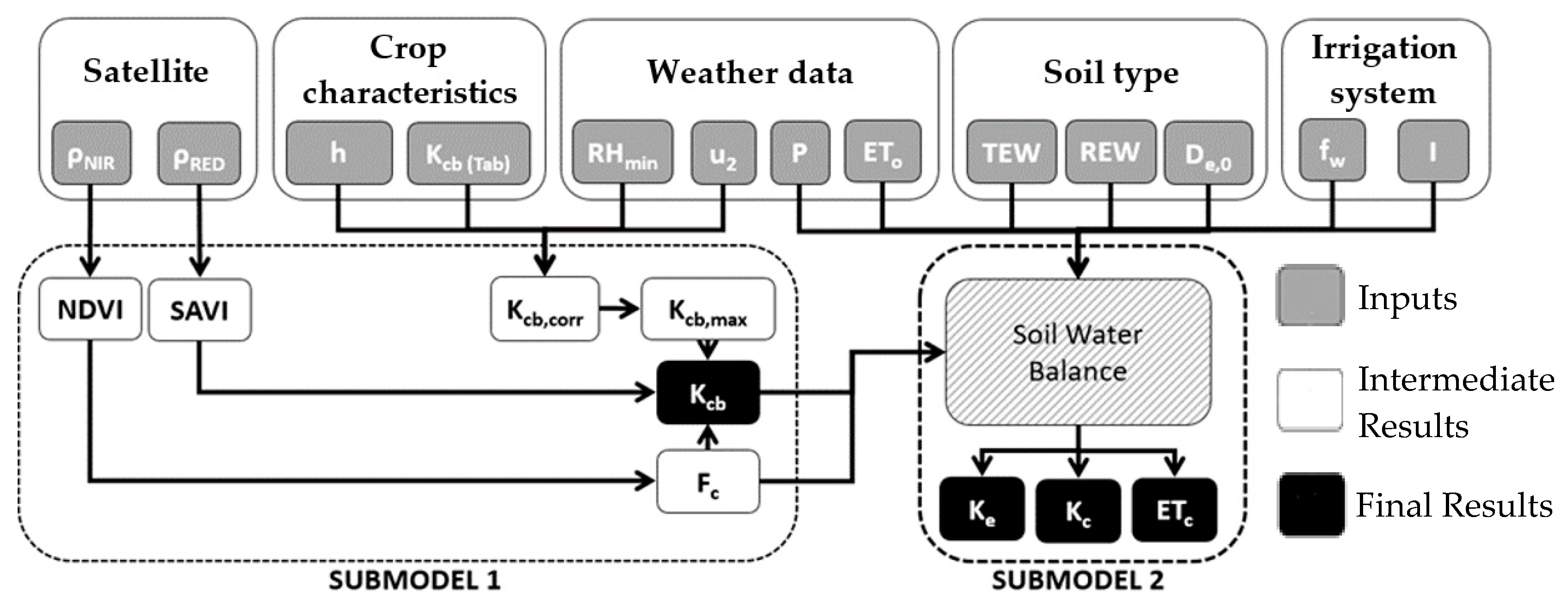
2.1. Model Theorical Framework

The dual K_c approach estimates the evapotranspiration of a given crop (ET_c) using the basal coefficient (K_cb), the evaporation coefficient (K_e), and the evapotranspiration of a reference surface (ET_o), defined as the water consumed by an extensive surface of green, well-watered grass of uniform height, actively growing and completely shading the ground [19].

ET_c = (K_cb + K_e) × ET_o

(1)

In this framework, K_cb is the ratio of ET_c over ET_o when the soil surface is dry but transpiration is occurring at a potential rate, that is, water is not limiting transpiration; whereas K_e refers to the soil evaporative component. The sum of both coefficients is known as the crop coefficient (K_c).

General K_cb values for the different seasonal stages of the main crops are tabulated [19], but refer to sub-humid climates with moderate wind speeds (e.g., minimum relative humidity of 45% and wind speeds of 2 m·s⁻¹, approximately). For those regions that do not meet these conditions, tabulated K_cb must be adjusted using the meteorological variables observed at those locations for correctly representing the local conditions [19].

In order to incorporate the spatial component into the estimation of K_c, the approach proposed in this study includes data derived from remote sensing imagery. More specifically, the model calculates two VI from bottom of atmosphere reflectivity values derived from satellite images: NDVI and SAVI. The first index, NDVI, allows for estimating the soil fraction covered by vegetation (F_c) through the linear, or approximately linear, relation between some VI and F_c in the range from bare soil to near full ground cover [30,31]. In addition, F_c in combination with SAVI, allows for correcting K_cb when non-homogeneous crops are considered [32].

K_cb = K_cb,max/F_c,max × ((SAVI − SAVI_min)/(SAVI_max − SAVI_min))

(2)

where the max and min subscripts refer to a high leaf area index (LAI) and a bare surface, respectively; and F_c,max is the vegetated covered fraction for which K_cb reaches its maximum value (K_cb,max). In this study, K_cb,max values were the FAO-56 tabulated values adjusted (K_cb,corr) for the local relative humidity and wind speed conditions (K_cb,corr in Figure 1) [19].

For the estimation of K_cb, the days when satellite images are not available (e.g., cloudy conditions or days without scheduled pass), the model extrapolates from the last available satellite image. Thus, for initial and mid stages, K_cb is assumed constant and, therefore, K_cb of a given day is considered equal to the K_cb value of the last available image. For development and final stages, the slope between the K_cb of the last available image and K_cb tabulated for mid and final stages, respectively, was determined.

In addition, K_e depends on the water available in the soil surface layer, which is computed as

K_e = K_r × (K_c,max − K_cb)

(3)

where K_c,max represents the maximum K_c value after an irrigation or precipitation event, and is calculated using the wind speed (u₂, m·s⁻¹), minimum relative humidity (RH_min, %), and crop height (h, m), as follows:

K_c,max = 1.2 + (0.04 × (u₂ − 2) − 0.004 × (RH_min − 45)) × (h/3)^0.3

(4)

K_r = (TEW − D_e)/(TEW − REW)

(5)

where TEW and REW are the total and the readily evaporable water, respectively (mm); and D_e represents the cumulative depletion from the soil surface layer (mm) estimated from a daily soil water balance.

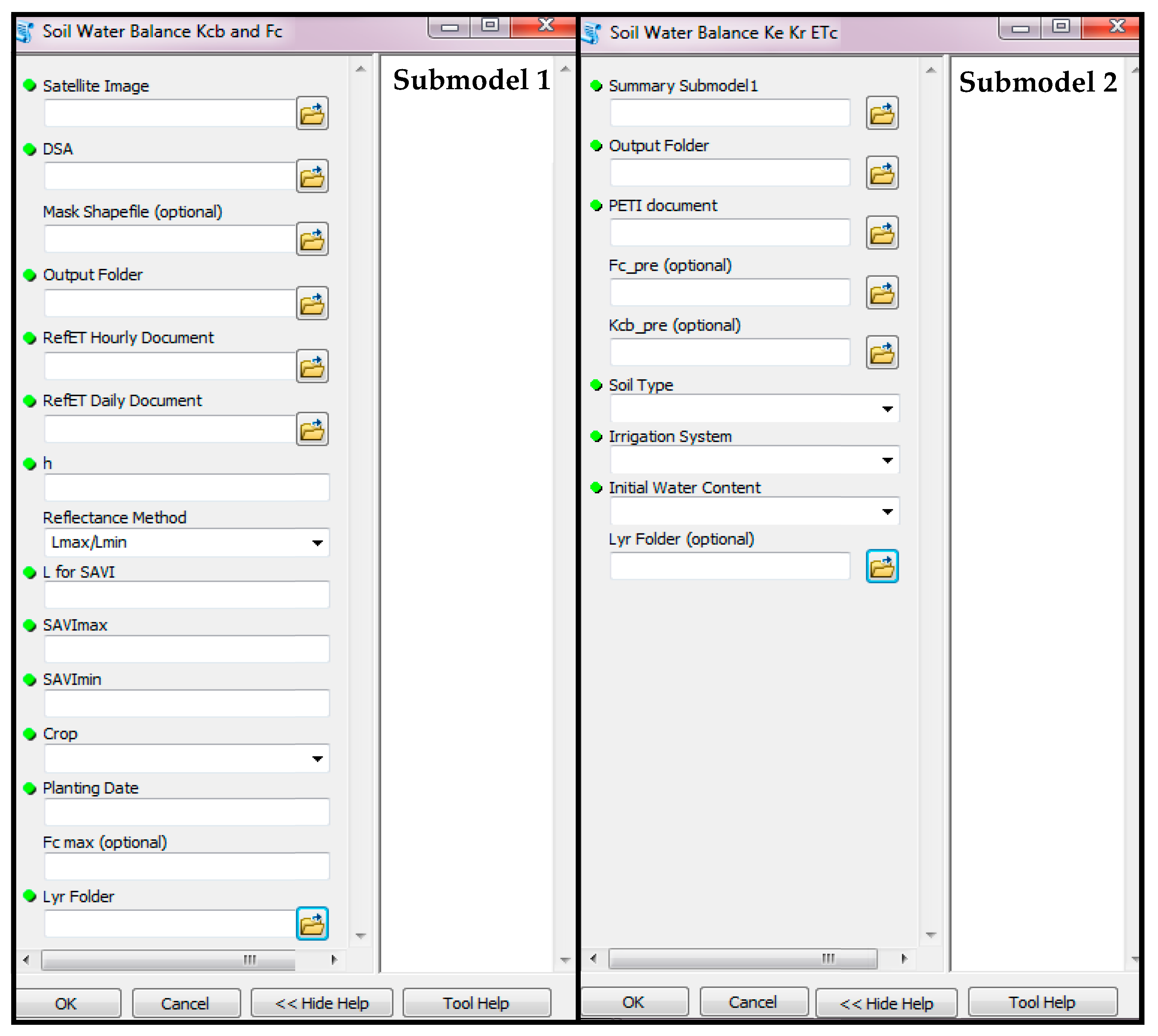
2.2. Model Implementation

The dual K_c model was implemented using ArcPy [33] because of its capacity for geographical data analysis, conversion and management, and map automation. This environment utilizes Python as a programming language. The model was split into two sub-models. The first one is intended for VIs, F_c, and K_cb computation, whereas the second one is focused on K_e, K_c, and ET_c estimation (Figure 1). Finally, the sub-model formulations were incorporated into an ArcGIS (v10.2; Esri, Redlands, CA, USA [33]) toolbox, which provides a friendly interface to execute the model, where the user only needs to select the values for the required inputs. The created tool was programmed for using images acquired from multiple satellites, identifying the source by the file name. This tool can be freely distributed to interested users by contacting the corresponding author.

2.3. Model Validation

The described model was validated in two sites: (i) a 1.32 ha lettuce orchard (Lactuca sativa L. cv. Little gem) located in Los Alcáceres, Murcia, southeast Spain (37°46′7′′ N, 0°50′13′′ W) during 2016; and (ii) a 3.56 ha peach orchard (Prunus persica L. Bastch cv. Amandina) located in Molina de Segura, Murcia, Southeast Spain (38°06′52′′ N, 1°12′46′′ W) during 2017. The lettuce planting date was 24 September and harvest took place on 11 November; therefore, the length of the crop growing cycle was 48 days. On the other hand, the peach orchard was planted in 2013 and the fruit harvest for 2017 occurred in May, followed by a long post-harvest period (namely, the peach cultivar is early maturing). Cloudless images from satellites Sentinel 2A, Landsat 7 and Landsat 8 collected during the studied growing seasons were considered as inputs. The spatial resolution of the images in the VNIR region was 10 m for Sentinel 2 and 30 m for Landsat 7 and 8, whereas the temporal resolution was 10 days for Sentinel 2A and 16 days for Landsat 7 and Landsat 8. Details about the different images used in this study are shown in

Table 1. Satellite imagery used for model validation during the lettuce growing season.

Date	Day of the Year	Satellite
29 September 2016	273	Landsat 8
7 October 2016	281	Landsat 7
8 October 2016	282	Sentinel 2A
15 October 2016	289	Landsat 8
23 October 2016	297	Landsat 7
31 October 2016	305	Landsat 8
7 November 2016	312	Sentinel 2A
8 November 2016	313	Landsat 7

and

Table 2. Satellite imagery used for model validation during the peach growing season.

Date	Day of the Year	Satellite
3 January 2017	3	Landsat 8
11 January 2017	11	Landsat 7
16 January 2017	16	Sentinel 2A
15 February 2017	46	Sentinel 2A
25 February 2017	56	Sentinel 2A
28 February 2017	59	Landsat 7
8 March 2017	67	Landsat 8
1 April 2017	91	Landsat 7
17 April 2017	107	Landsat 7
25 April 2017	115	Landsat 8
3 May 2017	123	Landsat 7
6 May 2017	126	Sentinel 2A
26 May 2017	146	Sentinel 2A
27 May 2017	147	Landsat 8
5 June 2017	156	Sentinel 2A
12 June 2017	163	Landsat 8
15 June 2017	166	Sentinel 2A
28 June 2017	179	Landsat 8
5 July 2017	186	Sentinel 2A
15 July 2017	196	Sentinel 2A
30 July 2017	211	Landsat 8
4 August 2017	216	Sentinel 2A
15 August 2017	227	Landsat 8
24 August 2017	236	Sentinel 2A

. A total of 8 and 23 cloudless satellite images were used for characterizing the lettuce and peach K_cb curves, respectively. They corresponded with the 73% (lettuce) and 45% (peach) of all satellite images acquired during the considered period. Only pure pixels, namely, those totally included in the plots, were considered for determining crop water demands in order to avoid edge-pixel contamination. In this sense, for the lettuce plot, the number of pure pixels was 6 and 99 for Landsat and Sentinel, respectively; whereas the number of pure pixels for the peach field was 23 and 291 for Landsat and Sentinel, respectively.

During the growing seasons, the plants were cultivated using standard practices in the area with a cumulative irrigation application of 120 mm and 293 mm for lettuce and peach, respectively. The total amounts of N, P₂O₅, and K₂O applied to fulfill the estimated crop nutrient demand were 56, 30, and 76 kg·ha⁻¹, respectively, for lettuce and 105, 85 and 192kg·ha⁻¹, respectively, for peach.

Lettuce crop height was measured weekly in 60 plants randomly distributed within the plot (

Table 3. Temporal evolution of lettuce height at the study site (average from 60 measurements per date and standard error, SE).

Date	Day of the Year	Height (cm) ± SE
29 September 2016	273	5.4 ± 0.18
6 October 2016	280	5.6 ± 0.13
13 October 2016	287	8.8 ± 0.12
20 October 2016	294	15.4 ± 0.16
27 October 2016	301	19.0 ± 0.18
3 November 2016	308	20.4 ± 0.25
9 November 2016	314	21.4 ± 0.26

), whereas the average peach height measured in the field was 2.40 m at the beginning of the year and was considered to be constant during the season. This information, as well as tabulated K_cb values [19], was incorporated into the model (h and K_{cb (Tab)} in Figure 1). The tabulated K_cb values for initial, mid, and end stages were 0.15, 0.90, and 0.90, respectively, for lettuce and 0.45, 0.85, and 0.60, respectively, for peach. Daily and hourly weather data, including air temperature, relative humidity, wind speed, precipitation, reference evapotranspiration (calculated using the Penman–Monteith equation [19]), and solar radiation (Figure 2 and Figure 3), were obtained from the nearest weather stations. The main utility of using hourly data is that this allows for a precise weather characterization at the satellite acquisition time. For the lettuce study site, the weather station considered was located 3 km from the experimental site at San Javier, Murcia (code TP22; http://siam.imida.es), whereas that for the peach site was located 1.5 km from the study site at Molina de Segura, Murcia (code MO22; http://siam.imida.es). Mean air temperature and relative humidity for the study period were 20.7 °C and 76.2%, and 18.57 °C and 54.23% for lettuce and peach, respectively; with a cumulative precipitation and ET_o of 30.2 and 120.9 mm, respectively, for lettuce, and 140.9 and 1002.2 mm, respectively, for peach (Figure 2 and Figure 3). Noticeably, only a few rainfall events greater than 5 mm occurred over both growing seasons and accounted for more than 80% of the total rainfall within the studied periods (Figure 2 and Figure 3). The values of TEW and REW were selected according to those defined in the FAO-56 document [19] for the different soils in both sites. More specifically, lettuce was grown on a loamy soil (sand 42%, silt 37; clay 21%), whereas the peach orchard was planted on a soil that was clay-loamy (sand 40%, silt 17%, clay 43%); corresponding with REW and TEW values of 9.0 and 19.0 mm, respectively, for lettuce and 9.5 and 24.5 mm, respectively, for peach. In addition, soil water balance was initialized at 15 September (day of year, DOY, 259) for lettuce and 15 January (DOY 15) for peach, because no significant precipitation events occurred during the previous weeks, allowing the assumption that all evaporable water had been depleted from the soil surface layer at the beginning of calculations, that is, D_{e, 0} = TEW.

2.4. Statistical Analyses

The comparison between K_cb values derived from the ArcGIS approach proposed in this study and those values tabulated in FAO-56 [19] was performed over the validation sites using the root mean square error (RMSE).

$$\mathrm{RMSE}=\sqrt{\frac{{{\displaystyle \sum }}_{\mathrm{l}=1}^{\mathrm{L}}{({\mathrm{K}}_{\mathrm{cb},\mathrm{FAO}56}-{\mathrm{K}}_{\mathrm{cb},\mathrm{estimated}})}^2}{\mathrm{L}}}$$

(6)

where K_{cb, FAO56} is the K_cb value derived from FAO-56; K_{cb, estimated} is the K_cb value estimated with the created tool, and L is the length of the crop season.

Considering that no other direct ET_c determination was available in the field sites, the tabulated FAO-56 values can be considered as a reasonable proxy for ET determinations because of their widespread use, particularly in herbaceous crops. The spatial variability within each plot was quantified by means of the coefficient of variation (CV) among the values of all pixels included in the studied fields:

$$\mathrm{CV}=\frac{\mathrm{SD}\times 100}{{\mathrm{K}}_{\mathrm{cb},\mathrm{mean}}}$$

(7)

where SD is the standard deviation within the plot and K_{cb, mean} is the average K_cb of all pixels included in the plot.

Additionally, the percent bias, PBIAS, was calculated to measure the average trend of the simulated data to be larger or smaller than the FAO-56 derived K_cb values.

$$\mathrm{PBIAS}=100\times \frac{{{\displaystyle \sum }}_{\mathrm{l}=1}^{\mathrm{L}}({\mathrm{K}}_{\mathrm{cb},\mathrm{estimated}}-{\mathrm{K}}_{\mathrm{cb},\mathrm{FAO}56})}{{{\displaystyle \sum }}_{\mathrm{l}=1}^{\mathrm{L}}{\mathrm{K}}_{\mathrm{cb},\mathrm{FAO}56}}$$

(8)

The optimal value of PBIAS is 0.0, with low-magnitude values indicating accurate model simulations. Positive values indicate overestimation, whereas negative values indicate model underestimation.

3. Results

3.1. Model Interface

Figure 4 shows the final interfaces for the different sub-models developed. On the left-hand side of each interface, the inputs required for running the model are listed. Thus, the required inputs for sub-model 1 and sub-model 2 are shown in

Table 4. Description of the different inputs considered in each sub-model. FAO—Food and Agricultural Organization of the United Nations; RefET—reference evapotranspiration; SAVI—soil-adjusted vegetation index; LAI—leaf area index.

Sub-model	Input	Description
Sub-model 1	Satellite Image	Folder containing the satellite image
	DSA	Three-band image where band 1 is digital elevation model; band 2 is slope; and band 3 is terrain aspect
	Mask Shapefile	Mask polygon delimitating the study area
	Output Folder	Folder where sub-model 1 outputs will be saved
	RefET Hourly Document	Hourly weather data as outputted by RefET software [34]
	RefET Daily Document	Daily weather data as outputted by RefET software [34]
	h	Crop height
	Reflectance Method	Method for calculating reflectance from radiance (for Landsat satellite images)
	L for SAVI	L parameter for SAVI calculation [35]. As default, this value is set to 0.5
	SAVImax	SAVI value corresponding with a high LAI surface
	SAVImin	SAVI value corresponding with a bare surface
	Crop	Crop under study
	Planting Date	Date when the crop was planted
	Fcmax	Vegetated covered fraction for which Kcb reaches its maximum value
	Lyr Folder	Folder containing the symbology for sub-model 1 outputs
Sub-model 2	Summary Submodel1	Text document automatically generated just after sub-model 1 has been run successfully
	Output Folder	Folder where sub-model 2 outputs will be saved
	PETI document	Text document including the daily irrigation amount applied to the crop
	Fc pre	Folder containing the vegetated covered fraction images of the previous days
	Kcb pre	Folder containing the Kcb images of the previous days
	Soil Type	Soil type category as defined in the FAO-56 document
	Irrigation System	Irrigation system as defined in the FAO-56 document
	Initial Water Content	Soil water content at the initialization of the soil water balance
	Lyr Folder	Folder containing the symbology for sub-model 2 outputs

. To help the user, a detailed description for each input is provided on the right-hand side of the interface when the mousepad icon is placed on each input box.

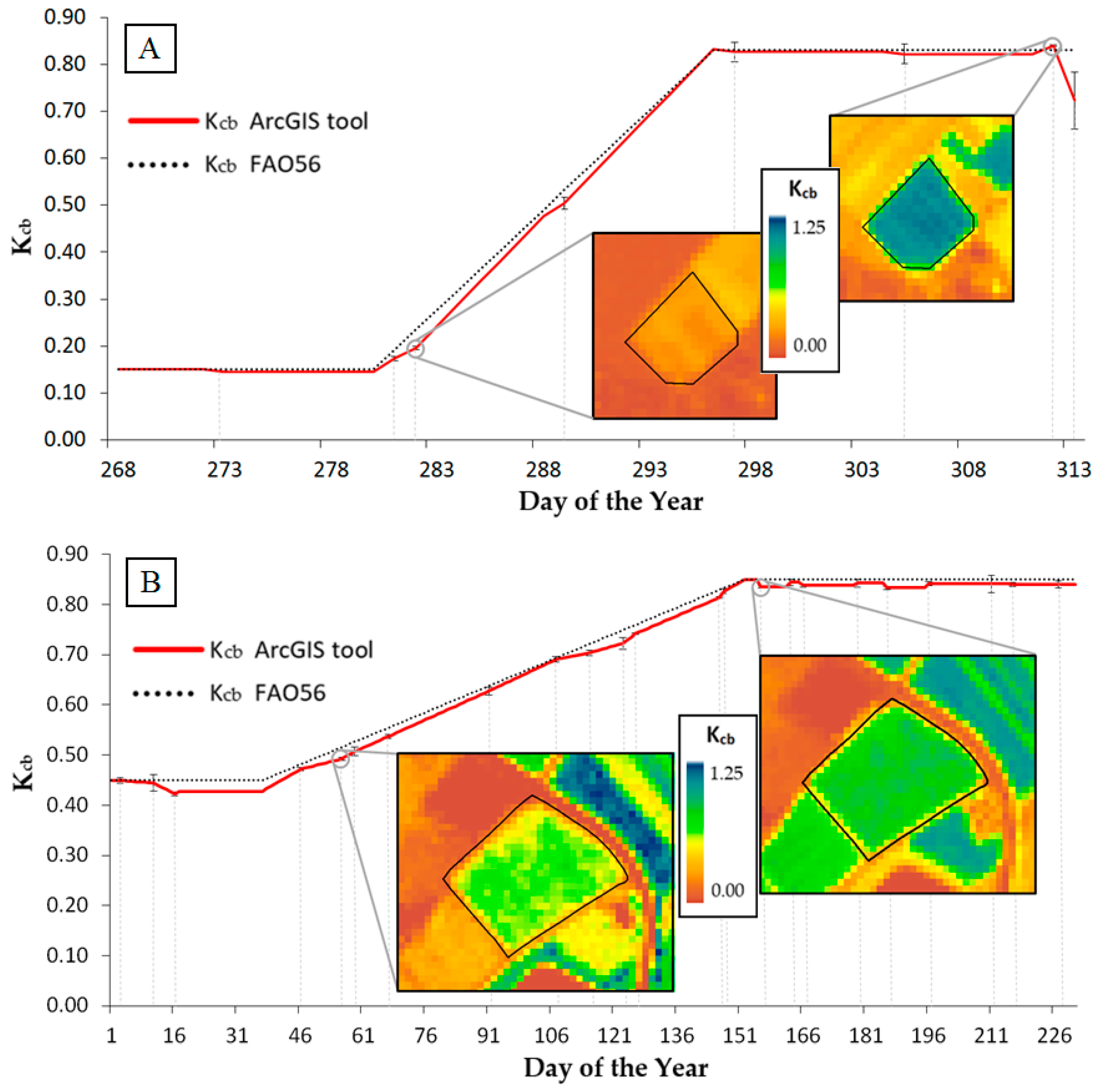
3.2. Practical Validation

Regarding the model validation, Figure 5 shows the temporal evolution of the K_cb values derived from the ArcGIS approach proposed in this study, as well as those values tabulated in FAO-56 [19], over the lettuce (Figure 5A) and peach growing seasons (Figure 5B). A good agreement between both K_cb values was obtained, as the RMSE (0.01–0.02) was low for both crops. The K_cb values estimated for lettuce were 0.15 and 0.85 for the initial and the mid-season stage, respectively, and values intermediate between these two for the crop-development stage. However, a slight underestimation (2.8% on average for the entire growing season) was observed in lettuce for the K_cb values obtained from the ArcGIS approach when compared with those derived from FAO-56, especially during the crop development stage (5.7% on average for the development stage; Figure 5A). For the peach orchard, K_cb values estimated were 0.43 and 0.84 for the initial and the mid-season stage, respectively, and values intermediate between these two for the crop-development stage. A slight underestimation was observed in peach for the K_cb values obtained from the ArcGIS approach when compared with those derived from FAO-56, with this being more evident during the initial and mid-season crop development stages (2.6% on average; Figure 5B). The reason for the lower underestimation observed in peach when compared with lettuce could be the higher frequency of available images used to build the K_cb curve (Figure 5). The PBIAS values obtained for lettuce and peach were −4.74% and −1.80%, respectively, confirming the underestimation pattern observed in Figure 5.

The K_cb variability within the lettuce field, assessed through CV, was low at the beginning of the growing season (CV ≈ 7.4%), increased during crop-development (CV ≈ 12.2%), and decreased again at the mid-season (CV ≈ 7.7%). For the peach orchard, CV was relatively high at the initial stage (CV ≈ 11.0%), and decreased during crop-development and mid-season stages (CV ≈ 4.7%). This variability could have been induced by the fact that our approach takes into account the actual soil surface covered by the crop (as determined by satellite images) for calculating K_cb, reflecting the uneven distribution of plant size for lettuce and the initial bud break for peach within the studied plots at the crop development and mid-season stages.

Examples of the spatially distributed K_cb output resulting from the application of the model for lettuce and peach at the development stage and at the end of the growing cycle (day of year (DOY) 282 and 312, respectively, for lettuce; and 56 and 156, respectively, for peach) are shown in Figure 5. The mean K_cb values on the lettuce plot were around 0.20 and 0.85 for DOY 282 and 312, respectively; whereas the mean K_cb values on the peach orchard were 0.50 and 0.84 for DOY 56 and 156, respectively. The reductions of K_cb near the field edges in both crops are the result of the pixel contamination due to the surrounding bare soil. This suggests that a larger pixel cut off could have reduced the errors.

4. Discussion

One main advantage of the tool developed here is that it does not require many inputs, and those compulsory for running the model are readily available, making its use easier. This solves the over-parameterization issue, which is one of the main limitations for using models for practical applications in agriculture [36,37]. In fact, after a certain level, an increase in model structure complexity does not necessarily lead to better estimations [38,39]. In this sense, the tool proposed here was able to provide reliable estimations of crop water demands using a set of easily available parameters; this capability, along with its friendly interface, might favor the use of the tool by farmers and technicians. In its present form, the toolbox is implemented using ArcGIS because of the flexibility offered by this commercial software. In the future, other software developers might take advantage of the algorithm details described here to migrate the toolbox into other open-software systems such as Quantum Geographical Information System (QGIS), expanding the operational possibilities of the tool developed here.

In addition, the integration of remote sensing technology into the tool permits obtaining a spatial representation of the crop water demand variability over a given plot or orchard and, therefore, it will be possible to apply a different irrigation scheduling to a given sector within the field [40,41,42,43]. This is the main improvement of our tool when compared with other approaches. Indeed, remote sensing technology has been incorporated into some DSS platforms (System of Participatory Information, Decision-support, and Expert knowledge for River-basin management, SPIDER [27]; Automated Radiative Transfer Models Operator, ARTMO [44]; AquaGIS [45]; Online Professional Irrigation Scheduling; Flexible and PrecIse IrriGation PlAtform to Improve FaRm Scale Water PrOductivity, FIGARO [46]). Some of these platforms are still ongoing developments, while some others provide information about other aspects of plant physiology and not directly on crop water requirements. To date, AquaGIS has been employed for simulating multi-year wheat yields under several irrigation strategies [45], proving the applicability of this approach for managing irrigation in large areas. However, AquaGIS is based on AquaCrop, a model that requires a higher number of inputs and parameters than the one implemented in the toolbox described in the current study. Therefore, our approach reduced model complexity when compared with AquaGIS. Other DSS, such as ARTMO [44], simulate and estimate vegetation structure or radiative transfer from vegetal canopies, with no regards to irrigation scheduling and, therefore, they have to be used by experts in order to gather the information provided by these platforms and translate it into irrigation strategies to be applied in the field. Another example of DSS with a module for irrigation scheduling is FIGARO [46], which also uses AquaCrop for determining crop water requirements, and has been applied only to field crops such as cotton [47]. In summary, our approach is easier to use than current platforms because it is more intuitive and requires a lower number of parameters and inputs; moreover, it is easily adapted to a great number of crop species, as long as their crop coefficients are available, as exemplified for lettuce (herbaceous plant) and peach (woody perennial species) in the current manuscript.

Furthermore, most of the available applications intended for crop management do not consider the spatial component, providing only numerical outputs and neglecting the spatial variability within the field [8,28,29,48,49,50]. Additionally, the tool proposed in this study allows for integrating information obtained from different satellites; improving the reliability and consistency of vegetation state variables; and, consequently, enhancing the estimations of crop water requirements [51,52,53,54]. Furthermore, the inclusion of the tool into a geographic information system (GIS) allows for task automation, which reduces computational time and permits modelling large areas at once, which is an important limitation in other models [11,12].

The validation with data for growing seasons of lettuce and peach in southeast Spain indicates that the proposed tool provides accurate crop water demand estimates when the FAO-56 methodology is taken as reference [19]. In this context, K_cb for lettuce is estimated at the crop development and mid-season stages in the current study as being from 0.6 to 0.85, which leads to K_c values similar to those measured in southeast Spain using Bowen ratio procedures, although slightly lower at the initial stage of crop development [25,55]. Regarding the peach orchard, K_cb values ranged from 0.45 (at the initial stage) to 0.85 (at the mid-season). The values at the initial stage were considerably higher than those proposed by other authors [56,57], whereas estimated K_cb values for mid stage were intermediate when compared with those previously reported [56,57]. This highlights the importance of the K_cb database used as input, which can clearly affect the model efficiency in estimating the actual ET_c. The period considered here covered the initial and mid stages, being necessary to enlarge the study until the leaf fall period to reach the K_cb value of the end season stage. It is necessary to develop and implement further new model routines, other than semi-empiric models, for computing ET, to be able to compute plant transpiration more specifically based on specific canopy resistance models. Additionally, the application of the proposed methodology allows the detection of the timing for bud break, complete canopy growth, and leaf senescence and fall. Nevertheless, a limitation with this type of crop is given by the spatial resolution of the satellite images, which does not allow distinguishing among orchard floor management practices. Moreover, outputs generated from the proposed tool collect K_cb spatial variations within the field, and this information can allow for precise irrigation management [58,59,60]; for instance, if the field has several irrigation sectors, they can be differently managed according to a possible uneven distribution of crop water requirements. In this sense, the uneven development of the crops within the field was reflected by the slight underestimation observed in the K_cb values derived from the tool, mainly during the crop development stage, which could have modified the SAVI and, therefore, the K_cb value. In contrast, the FAO-56 method employs a fixed value for fraction cover at a given developmental stage of the crop, irrespective of the SAVI, likely causing the underestimation of our approach when compared with the FAO-56 as a reference. Moreover, the FAO-56 K_cb values used compute crop water requirements under conditions of complete absence of biotic or abiotic stress and we cannot rule out the possibility that the experimental plants had temporarily suffered some slight limitations in their growth and development. In order to consider this issue, the next version of the developed tool will include the water stress coefficient, K_s [19]. Additionally, the temporal evolution of CV and RMSE showed that the variation observed was probably caused by the uneven distribution of plant sizes that left a variable surface of bare soil within the field. Once the crop started to develop, CV and RMSE increased, reflecting different growing rates of lettuce and peach canopies throughout the field. Finally, at mid-season, the variability decreased, probably because the crops reached a high-vegetated fraction cover and a more homogeneous distribution (for the case of lettuce) over the entire field. Furthermore, the selection of the pixels within the study area and the way the satellite images are cut off may cause additional errors for the estimation of crop water requirements at the edges of the field.

The implemented tool could be incorporated into a cloud-based DSS that allows for integrating data from various sources and, therefore, for assessing different scales ranging from small, single farms to large catchments; for centralizing the control of field devices; and for transforming the data into useful knowledge for decision making [61,62]. In this sense, potential applications might consider the estimation of the soil water content, which could be, for instance, of interest in humid areas where high soil moisture levels often hamper soil management using heavy tractors and machinery. The tool created can be also used in combination with weather forecasts as inputs instead of past weather data, which may allow for estimating future irrigation requirements and predicting the occurrence of extreme events [63,64,65]. Additionally, the satellite image download, pre-processing (e.g., radiometric, geometric, and atmospheric image corrections; cloud detection), and post-processing tasks are susceptible to being automatized, so that the results could be delivered to end-users (farmers, stakeholders, and policy makers) at near-real time, which facilitates the adoption of quick responses to agricultural issues [66].

Indeed, the proposed tool provides a user-friendly approach for the spatial estimation of crop water demands that can be incorporated into a DSS to generate real solutions for the agricultural sector in terms of irrigation scheduling and other applications related to the agro-ecosystem water balance.

References

1. Antle, J.M.; Jones, J.W.; Rosenzweig, C. Towards a new generation of agricultural system models, data, and knowledge products: Introduction. Agric. Syst. 2017, 155, 186–190. [Google Scholar] [CrossRef] [PubMed]
2. Donatelli, M.; Magarey, R.D.; Bregaglio, S.; Willocquet, L.; Whish, J.P.M.; Savary, S. Modelling the impacts of pests and diseases on agricultural systems. Agric. Syst. 2017, 155, 213–224. [Google Scholar] [CrossRef] [PubMed]
3. Zarco-Tejada, P.J.; Camino, C.; Beck, P.S.A.; Calderon, R.; Hornero, A.; Hernández-Clemente, R.; Kattenborn, T.; Montes-Borrego, M.; Susca, L.; Morelli, M.; et al. Previsual symptoms of Xylella fastidiosa infection revealed in spectral plant-trait alterations. Nat. Plants 2018, 4, 432–439. [Google Scholar] [CrossRef] [PubMed]
4. Le Bot, J.; Adamowicz, S.; Robin, P. Modelling plant nutrition of horticultural crops: A review. Sci. Hortic. 1998, 74, 47–82. [Google Scholar] [CrossRef]
5. Ransom, K.M.; Nolan, B.T.; Traum, J.A.; Faunt, C.C.; Bell, A.M.; Gronberg, J.A.M.; Wheeler, D.C.; Rosecrans, C.Z.; Jurgens, B.; Schwarz, G.E.; et al. A hybrid machine learning model to predict and visualize nitrate concentration throughout the Central Valley aquifer, California, USA. Sci. Total Environ. 2017, 601–602, 1160–1172. [Google Scholar] [CrossRef] [PubMed]
6. Rosa, R.D.; Paredes, P.; Rodrigues, G.C.; Alves, I.; Fernando, R.M.; Pereira, L.S.; Allen, R.G. Implementing the dual crop coefficient approach in interactive software. 1. Background and computational strategy. Agric. Water Manag. 2012, 103, 8–24. [Google Scholar] [CrossRef]
7. Pereira, L.S.; Allen, R.G.; Smith, M.; Raes, D. Crop evapotranspiration estimation with FAO56: Past and future. Agric. Water Manag. 2015, 147, 4–20. [Google Scholar] [CrossRef]
8. Steduto, P.; Hsiao, T.C.; Raes, D.; Fereres, E. AquaCrop: The FAO Crop Model to Simulate Yield Response to Water: I. Concepts and Underlying Principles. Agron. J. 2009, 101, 426–437. [Google Scholar] [CrossRef]
9. Lobell, D.B.; Burke, M.B. On the use of statistical models to predict crop yield responses to climate change. Agric. For. Meteorol. 2010, 150, 1443–1452. [Google Scholar] [CrossRef]
10. Janssen, J.C.; Porter, C.H.; Moore, A.D.; Athanasiadis, I.N.; Foster, I.; Jones, J.W.; Antle, J.M. Towards a new generation of agricultural system data, models and knowledge products: Information and communication technology. Agric. Syst. 2017, 155, 200–212. [Google Scholar] [CrossRef]
11. Jones, J.W.; Antle, J.M.; Basso, B.; Boote, K.J.; Conant, R.T.; Foster, I.; Godfray, H.C.J.; Herrero, M.; Howitt, R.E.; Janssen, S.; et al. Brief history of agricultural systems modeling. Agric. Syst. 2016, 155, 240–254. [Google Scholar] [CrossRef] [PubMed]
12. Ding, Y.; Wang, L.; Li, Y.; Li, D. Model predictive control and its application in agriculture: A review. Comput. Electron. Agric. 2018, 151, 104–117. [Google Scholar] [CrossRef]
13. Anderson, M.C.; Kustas, W.P.; Norman, J.M. Upscaling and downscaling—A regional view of the Soil-Plant-Atmosphere continuum. Agron. J. 2003, 95, 1408–1423. [Google Scholar] [CrossRef]
14. Ramírez-Cuesta, J.M.; Allen, R.G.; Zarco-Tejada, P.J.; Kilic, A.; Santos, C.; Lorite, I.J. Impact of the spatial resolution on the energy balance components on an open-canopy olive orchard. Int. J. Appl. Earth Obs. Geoinf. 2019, 74, 88–102. [Google Scholar] [CrossRef]
15. Crago, R.D.; Brutsaert, W. Conservation and variability of the evaporative fraction during the daytime. J. Hydrol. 1996, 180, 173–194. [Google Scholar] [CrossRef]
16. Allen, R.G.; Tasumi, M.; Morse, A.; Trezza, R.; Wright, J.L.; Bastiaanssen, W.; Kramber, W.; Lorite, I.; Robison, C.W. Satellite-Based Energy Balance for Mapping Evapotranspiration with Internalized Calibration (METRIC)-Applications. J. Irrig. Drain. Eng. 2007, 133, 395–406. [Google Scholar] [CrossRef]
17. Aguilar, A.L.; Flores, H.; Crespo, G.; Marín, M.I.; Campos, I.; Calera, A. Performance assessment of MOD16 in evapotranspiration evaluation in Northwestern Mexico. Water 2018, 10, 901. [Google Scholar] [CrossRef]
18. Mateos, L.; González-Dugo, M.P.; Testi, L.; Villalobos, F.J. Monitoring evapotranspiration of irrigated crops using crop coefficients derived from time series of satellite images. I. Method validation. Agric. Water Manag. 2013, 125, 81–91. [Google Scholar] [CrossRef]
19. Allen, R.G.; Pereira, L.S.; Raes, D.; Smith, M. Crop Evapotranspiration: Guidelines for Computing Crop Water Requirements; FAO Irrigation and Drainage Paper No. 56; Food and Agriculture Organization of the United Nations: Rome, Italy, 1998. [Google Scholar]
20. Er-Raki, S.; Chehbouni, A.; Boulet, G.; Williams, D.G. Using the dual approach of FAO-56 for partitioning ET into soil and plant components for olive orchards in a semi-arid region. Agric. Water Manag. 2010, 97, 1769–1778. [Google Scholar] [CrossRef] [Green Version]
21. Paço, T.A.; Ferreira, M.I.; Rosa, R.D.; Paredes, P.; Rodrigues, G.C.; Conceição, N.; Pacheco, C.A.; Pereira, L.S. The dual crop coefficient approach using a density factor to simulate the evapotranspiration of a peach orchard: SIMDualKc model vs. eddy covariance measurements. Irrig. Sci. 2012, 30, 115–126. [Google Scholar] [CrossRef]
22. Consoli, S.; Vanella, D. Mapping crop evapotranspiration by integrating vegetation indices into a soil water balance model. Agric. Water Manag. 2014, 143, 71–81. [Google Scholar] [CrossRef]
23. Katerji, N.; Rana, G. FAO-56 methodology for determining water requirement of irrigated crops: Critical examination of the concepts, alternative proposals and validation in Mediterranean region. Theor. Appl. Climatol. 2014, 116, 515–536. [Google Scholar] [CrossRef]
24. Allen, R.G.; Pereira, L.S.; Smith, M.; Raes, D.; Wright, J.L. FAO-56 Dual Crop Coefficient Method for Estimating Evaporation from Soil and Application Extensions. J. Irrig. Drain. Eng. 2005, 131, 2–13. [Google Scholar] [CrossRef] [Green Version]
25. Fernández-Pacheco, D.G.; Escarabajal-Henajeros, D.; Ruiz Canales, A.; Conesa, J.; Molina-Martínez, J.M. A digital image-processing-based method for determining the crop coefficient of lettuce crops in the southeast of Spain. Biosyst. Eng. 2014, 117, 23–34. [Google Scholar] [CrossRef]
26. Jones, J.W.; Hoogenboom, G.; Porter, C.H.; Boote, K.J.; Batchelor, W.D.; Hunt, L.A.; Wilkens, P.W.; Singh, U.; Gijsman, A.J.; Ritchie, J.T. The DSSAT Cropping System Model. Eur. J. Agron. 2003, 18, 235–265. [Google Scholar] [CrossRef]
27. Moreno-Rivera, J.M.; Calera, A.; Osann, A. SPIDER—An Open GIS application use case. In Proceedings of the Open GIS UK Conference, Nottingham, UK, 22 June 2009. [Google Scholar]
28. Navarro-Hellín, H.; Martínez-del-Rincon, J.; Domingo-Miguel, R.; Soto-Valles, F.; Torres-Sánchez, R. A decision support system for managing irrigation in agriculture. Comput. Electron. Agric. 2016, 124, 121–131. [Google Scholar] [CrossRef] [Green Version]
29. Li, H.; Li, J.; Shen, Y.; Zhang, X.; Lei, Y. Web-based irrigation decision support system with limited inputs for farmers. Agric. Water Manag. 2018, 210, 279–285. [Google Scholar] [CrossRef]
30. Huete, A.R.; Jackson, R.D.; Post, D.F. Spectral response of a plant canopy with different soil backgrounds. Remote Sens. Environ. 1985, 17, 37–53. [Google Scholar] [CrossRef]
31. Ormsby, J.P.; Choudhury, B.J.; Owe, M. Vegetation spatial variability and its effect on vegetation indices. Int. J. Remote Sens. 1987, 8, 1301–1306. [Google Scholar] [CrossRef]
32. González-Dugo, M.P.; Neale, C.M.U.; Mateos, L.; Kustas, W.P.; Prueger, J.H.; Anderson, M.C.; Li, F. A Comparison of Operational Remote Sensing-Based Models for Estimating Crop Evapotranspiration. Agric. For. Meteorol. 2009, 149, 1843–1853. [Google Scholar] [CrossRef]
33. ESRI. ArcGIS for Desktop; Version 10.2; Environmental Systems Research Institute: Redlands, CA, USA, 2014; Available online: http://www.esri.com/ (accessed on 23 December 2018).
34. Allen, R.G. Ref-ET: Reference Evapotranspiration Calculation Software for FAO and ASCE Standardized Equations; University of Idaho: Kimberly, ID, USA, 2010. [Google Scholar]
35. Huete, A.R. A soil adjusted vegetation index (SAVI). Remote Sens. Environ. 1988, 25, 295–309. [Google Scholar] [CrossRef]
36. Reichert, P.; Omlin, M. On the usefulness of overparameterized ecological models. Ecol. Model. 1997, 95, 289–299. [Google Scholar] [CrossRef]
37. Perrin, C.; Michel, C.; Andréassian, V. Does a large number of parameters enhance model performance? Comparative assessment of common catchment model structures on 429 catchments. J. Hydrol. 2001, 242, 275–301. [Google Scholar] [CrossRef]
38. Loague, K.M.; Freeze, R.A. A comparison of rainfall-runoff modelling techniques on small upland catchments. Water Resour. Res. 1985, 21, 229–248. [Google Scholar] [CrossRef]
39. Bastidas, L.A.; Hogue, T.S.; Sorooshian, S.; Gupta, H.V.; Shuttleworth, W.J. Parameter sensitivity analysis for different complexity land surface models using multicriteria methods. J. Geophys. Res. 2006, 111, D20101. [Google Scholar] [CrossRef]
40. Belaqziz, S.; Khabba, S.; Er-Raki, S.; Jarlan, L.; Le Page, M.; Kharrou, M.H.; El Adnani, M.; Chehbouni, A. A new irrigation priority index based on remote sensing data for assessing the networks irrigation scheduling. Agric. Water Manag. 2013, 119, 1–9. [Google Scholar] [CrossRef]
41. González-Dugo, V.; Zarco-Tejada, P.J.; Nicolás, E.; Nortes, P.A.; Alarcón, J.J.; Intrigliolo, D.S.; Fereres, E. Using high resolution UAV thermal imagery to assess the variability in the water status of five fruit tree species within a commercial orchard. Precis. Agric. 2013, 14, 660–678. [Google Scholar] [CrossRef]
42. Bellvert, J.; Zarco-Tejada, P.J.; Marsal, J.; Girona, J.; González-Dugo, V.; Fereres, E. Vineyard irrigation scheduling based on airborne thermal imagery and water potential thresholds. Aust. J. Grape Wine Res. 2016, 22, 307–315. [Google Scholar] [CrossRef]
43. Romero, M.; Luo, Y.; Su, B.; Fuentes, S. Vineyard water status estimation using multispectral imagery from an UAV platform and machine learning algorithms for irrigation scheduling management. Comput. Electron. Agric. 2018, 147, 109–117. [Google Scholar] [CrossRef]
44. Verrelst, J.; Romijn, E.; Kooistra, L. Mapping vegetation density in a heterogeneous river floodplain ecosystem using pointable CHRIS/PROBA data. Remote Sens. 2012, 4, 2866–2889. [Google Scholar] [CrossRef]
45. Lorite, I.J.; García-Vila, M.; Santos, C.; Ruiz-Ramos, M.; Fereres, E. AquaData and AquaGIS: Two Computer Utilities for Temporal and Spatial Simulations of Water-Limited Yield with AquaCrop. Comput. Electron. Agric. 2013, 96, 227–237. [Google Scholar] [CrossRef]
46. Simionesei, L.; Galvão, P.; Ramos, T.B.; Leitão, P.C.; Silva, A.; Neves, R. A plataforma FIGARO no apoio à gestão da rega. In Proceedings of the Livro de Actas do VII Congresso Ibérico das Ciências do Solo e do VI Congresso de Rega e Drenagem Solos e Água: Fontes (esgotáveis) de vida e de desenvolvimento, Beja, Portugal, 13–15 September 2016; pp. 309–312. (In Portuguese). [Google Scholar]
47. Tsakmakis, I.; Kokkos, N.; Pisinaras, V.; Papaevangelou, V.; Hartzigiannakis, E.; Arampatzis, G.; Gikas, G.D.; Linker, R.; Zoras, S.; Evagelopoulos, V.; et al. Operational precise irrigation for cotton cultivation through the coupling of meteorological and crop growth models. Water Resour. Manag. 2017, 31, 563–580. [Google Scholar] [CrossRef]
48. Thysen, I.; Detlefsen, N.K. Online decision support for irrigation for farmers. Agric. Water Manag. 2006, 86, 269–276. [Google Scholar] [CrossRef]
49. Giusti, E.; Marsili-Libelli, S. A Fuzzy Decision Support System for irrigation and water conservation in agriculture. Environ. Model. Softw. 2015, 63, 73–86. [Google Scholar] [CrossRef]
50. Yang, G.; Liu, L.; Guo, P.; Li, M. A flexible decision support system for irrigation scheduling in an irrigation district in China. Agric. Water Manag. 2017, 179, 378–389. [Google Scholar] [CrossRef]
51. Corbari, C.; Bissolati, M.; Mancini, M. Multi-scales and multi-satellites estimates of evapotranspiration with a residual energy balance model in the Muzza agricultural district in Northern Italy. J. Hydrol. 2015, 524, 243–254. [Google Scholar] [CrossRef]
52. Mousivand, A.; Menenti, M.; Gorte, B.; Verhoef, W. Multi-temporal, multi-sensor retrieval of terrestrial vegetation properties from spectral–directional radiometric data. Remote Sens. Environ. 2015, 158, 311–330. [Google Scholar] [CrossRef]
53. Semmens, K.A.; Anderson, M.C.; Kustas, W.P.; Gao, F.; Alfieri, J.G.; McKee, L.; Prueger, J.H.; Hain, C.R.; Cammalleri, C.; Yang, Y.; et al. Monitoring daily evapotranspiration over two California vineyards using Landsat 8 in a multi-sensor data fusion approach. Remote Sens. Environ. 2016, 185, 155–170. [Google Scholar] [CrossRef] [Green Version]
54. Fieuzal, R.; Baup, F. Forecast of wheat yield throughout the agricultural season using optical and radar satellite images. Int. J. Appl. Earth Obs. Geoinf. 2017, 59, 147–156. [Google Scholar] [CrossRef]
55. González-Esquiva, J.M.; García-Mateos, G.; Escarabajal-Henajeros, D.; Hernández-Hernández, J.L.; Ruiz-Canales, A.; Molina-Martínez, J.M. A new model for water balance estimation on lettuce crops using effective diameter obtained with image analysis. Agric. Water Manag. 2017, 183, 116–122. [Google Scholar] [CrossRef]
56. Ayars, J.E.; Johnson, R.S.; Phene, C.J.; Trout, T.J.; Clark, D.A.; Mead, R.M. Water use by drip-irrigated late-season peaches. Irrig. Sci. 2003, 22, 187–194. [Google Scholar] [CrossRef]
57. Abrisqueta, I.; Abrisqueta, J.M.; Tapia, L.M.; Munguía, J.P.; Conejero, W.; Vera, J.; Ruiz-Sánchez, M.C. Basal crop coefficients for early-season peach trees. Agric. Water Manag. 2013, 121, 158–163. [Google Scholar] [CrossRef]
58. Lee, W.S.; Alchanatis, V.; Yang, C.; Hirafuji, M.; Moshou, D.; Li, C. Sensing technologies for precision specialty crop production. Comput. Electron. Agric. 2010, 74, 2–33. [Google Scholar] [CrossRef]
59. Gago, J.; Douthe, C.; Coopman, R.E.; Gallego, P.P.; Ribas-Carbo, M.; Flexas, J.; Escalona, J.; Medrano, H. UAVs challenge to assess water stress for sustainable agriculture. Agric. Water Manag. 2015, 153, 9–19. [Google Scholar] [CrossRef]
60. Khanal, S.; Fulton, J.; Shearer, S. An overview of current and potential applications of thermal remote sensing in precision agriculture. Comput. Electron. Agric. 2017, 139, 22–32. [Google Scholar] [CrossRef]
61. Sørensen, C.; Pesonen, L.; Bochtis, D.; Vougioukas, S.; Suomi, P. Functional requirements for a future farm management information system. Comput. Electron. Agric. 2011, 76, 266–276. [Google Scholar] [CrossRef]
62. Tan, L. Cloud-based decision support and automation for precision agriculture in orchards. IFAC-PapersOnLine 2016, 49, 330–335. [Google Scholar] [CrossRef]
63. Cabelguenne, M.; Debaeke, Ph.; Puech, J.; Bose, N. Real time irrigation management using the EPIC-PHASE model and weather forecasts. Agric. Water Manag. 1997, 32, 227–238. [Google Scholar] [CrossRef]
64. Bergez, J.E.; Garcia, F. Is it worth using short-term weather forecasts for irrigation management? Eur. J. Agron. 2010, 33, 175–181. [Google Scholar] [CrossRef]
65. Lorite, I.J.; Ramírez-Cuesta, J.M.; Cruz-Blanco, M.; Santos, C. Using weather forecast data for irrigation scheduling under semi-arid conditions. Irrig. Sci. 2015, 33, 411–427. [Google Scholar] [CrossRef]
66. Zhao, R.-X.; Kou, Y.-T.; Xian, G.-J.; Mao, G.-W. Study on Technologies for Information Monitoring and Quick Response of Agricultural Focuses and Significant Events. Agric. Sci. China 2010, 9, 764–770. [Google Scholar] [CrossRef]
Figure 1. Flowchart of the dual Kc model implemented into ArcPy, showing the inputs, intermediate results, and outputs. ρNIR and ρRED are the reflectances corresponding to the infrared and red bands, respectively; fw is the fraction of soil surface wetted by irrigation; and I is the irrigation depth on each day that infiltrates the soil (mm). For definitions of the rest of abbreviations used in the figure, readers are referred to the main text.
Water 11 00038 g001
Figure 2. Daily weather data obtained from the weather station located at San Javier, Murcia (code TP22; http://siam.imida.es) for the period including the lettuce growing season in 2016. Abbreviations: Prec = precipitation; Tmean = mean temperature; Tmax = maximum temperature; Tmin = minimum temperature; RH = relative humidity; u2 = wind speed; ETo = reference evapotranspiration; SR = solar radiation.
Water 11 00038 g002
Figure 3. Daily weather data obtained from the weather station located at Molina de Segura, Murcia (code MO22; http://siam.imida.es) for the period including the peach growing season in 2017. Abbreviations: Prec = precipitation; Tmean = mean temperature; Tmax = maximum temperature; Tmin = minimum temperature; RH = relative humidity; u2 = wind speed; ETo = reference evapotranspiration; SR = solar radiation.
Water 11 00038 g003
Figure 4. Toolbox interfaces of sub-model 1 (left) and sub-model 2 (right) implemented in ArcGIS (geographic information system), showing the different input parameters (Table 4 provides explanations for each item). RefET—reference ET; DSA—digital elevation model, slope, and terrain aspect; SAVI—soil-adjusted vegetation index.
Water 11 00038 g004
Figure 5. Temporal evolution of the Kcb values obtained from the developed ArcGIS tool and those derived from the Food and Agricultural Organization of the United Nations (FAO)-56 document for lettuce ((A): Coordinates 37°46′7′′ N, 0°50′13′′ W) and peach (B): Coordinates 38°06′52′′ N, 1°12′46′′ W); and examples of the resultant Kcb images for different crop stages. Error bars represent the standard error (SE) within the field.)
Water 11 00038 g005