A Coupled Model for Simulating Water and Heat Transfer in Soil-Plant-Atmosphere Continuum with Crop Growth


1
Center for Agricultural Water Research in China, College of Water Resources & Civil Engineering, China Agricultural University, Beijing 10083, China
2
Institute for Infrastructure and Environment, Heriot-Watt University, Edinburgh EH14 4AS, UK
*
Author to whom correspondence should be addressed.
Water 2019, 11(1), 47; https://doi.org/10.3390/w11010047
Submission received: 17 November 2018
/
Revised: 19 December 2018
/
Accepted: 21 December 2018
/
Published: 28 December 2018
(This article belongs to the Section Water Use and Scarcity)
Abstract
:Crop growth is influenced by the energy partition and water–heat transfer in the soil and canopy, while crop growth affects the land surface energy distribution and soil water-heat dynamics. In order to simulate the above processes and their interactions, a new model, named CropSPAC, was developed considering both the growth of winter wheat and the water–heat transfer in Soil-Plant-Atmosphere Continuum (SPAC). In CropSPAC, the crop module depicts the dynamic changes of leaf area index (LAI), crop height, and the root distribution and outputs them to the SPAC module, while the latter outputs soil moisture conditions for the crop module. CropSPAC was calibrated and validated by field experiment of winter wheat in Yongledian, Beijing, with five levels of irrigation treatments, namely W0 (0 mm), W1 (60 mm), W2 (110 mm), W3 (170 mm), and W4 (230 mm). Results show that CropSPAC could predict the soil water and temperature distribution, and winter wheat growth with acceptable accuracy. For example, for the 0–1 m soil water storage, the R2 for W0, W1, W2, W3, and W4 is 0.90, 0.88, 0.90, 0.91, and 0.79, and the root mean square error (RMSE) is 17.24 mm, 27.65 mm, 20.47 mm, 22.35 mm, and 12.88 mm, respectively. For soil temperature along the soil profile, the R2 ranges between 0.96 and 0.98, and the RMSE between 1.22 °C and 1.94 °C. For LAI, the R2 varied from 0.76 to 0.96, and the RMSE from 0.52 to 0.67. We further compared the simulation results by CropSPAC and its two detached modules, i.e., crop and the SPAC modules. Results demonstrate that the coupled model could better reflect the interactions between crop growth and soil moisture condition, more suitable to be used under deficit irrigation conditions.
1. Introduction
Crop habitat, including the water and heat conditions in the soil root zone and crop canopy, is crucial for crop growth and yield formation. Plants extract water from soil, transport water within xylem vessels, and lose water by transpiration through stomata in plant leaves [1]. Transpiration flux provides the driving force to capture nutrients from the soil. By absorbing the energy in solar radiation, crop photosynthesis could be accomplished which produce carbohydrate for biomass accumulation and distribution [2]. Additionally, the surrounding temperature is a vital signal for determining the crop phenological period. On the other hand, crop growth conditions also affect crop habitats by influencing the land surface energy distribution, partition of solar energy, and root zone development and water uptake, etc. [3]. Understanding their interactions is essential for scientific management of farmland, especially in conditions with great changes in farmland soil moisture and heat (such as deficit irrigation, greenhouses, coverage, etc.), so as to provide guidance for enhancing the crop yields and water use efficiency (WUE).
Crop models were commonly used for quantitative description of the crop growth process, which can also interpret experimental results [4], and as agronomic research tools for crop production management [5,6], land resource evaluation, and agricultural production impact assessment [7,8]. Additionally, crop models have also been used to assess and develop irrigation scheduling strategies under limited available water for increasing crop water productivity [9,10]. Examples of such models that have been used for crop production systems include EPIC [11], WOFOST [12], DNDC [13], DSSAT [14], and AquaCrop [15], etc.
Current crop models normally did not include the influence of energy partitioning on the crop growth and water consumption. However, under the circumstances of deficit irrigation or film mulching, which had been extensively applied in North and Northwest China, it has profound influence on the latent heat consumption through soil surface evaporation, thus affecting the energy partition and the advancement of crop growth stage and the crop water consumption [16]. Therefore, a model that could describe not only the crop growth, but also the energy partition, and the water and heat transfer in the soil and canopy, should be more suitable under such circumstances.
Philips [17] proposed the concept of the Soil-Plant-Atmosphere Continuum (SPAC), considering the water movement in the SPAC system as a continuous process. Based on this concept, the water–heat transfer in SPAC describes the process of the water and heat movement in the soil, moisture, and heat transfer in the canopy, as well as the energy partition and consumption in the soil surface and canopy [18], which is essential for crop growth, formation of yield, and a key subject in agriculture, hydrology, and atmospheric science [19]. SPAC theory laid a theoretical foundation for the study of modern farmland water, which has prompted many researchers to conduct in-depth studies in this field [20,21,22]. Software for simulating the water and heat exchanges near land surface were also developed under this concept, e.g., SWAP [23], for simulating the vertical transport of water, solutes, and heat in variably saturated, cultivated soils, SWAT [24], for assessing the impact of management on water supplies and nonpoint source pollution in watersheds and large river basins, and land surface model (LSMs), for simulating surface energy, water fluxes, and surface energy and water budgets in response to near-surface atmospheric forcing [25,26].
In SPAC model the plant variables was generally considered as static parameters, such as leaf area index (LAI), which was just an input data to drive SPAC model simulation. Those input data were usually obtained from field experiment or literature and did not change with the calculated water and heat condition in SPAC. Actually, the crop growth indices, as the output of the crop model, should be expected to have a noticeable impact on the water–heat transfer in the SPAC system, such as root uptake from the soil and water lost to the atmosphere through transpiration. On the other hand, the crop growth was affected by radiation, temperature, and humidity of the atmosphere, soil water, etc., which was the output of SPAC water–heat transfer model.
Given the limitations of previous crop models and SPAC models as outlined above, it is necessary to develop a new model in which both the growth of crop, the water–heat transfer in SPAC and the interactions between them should be considered. Crop index from crop models provides input data for SPAC, while SPAC provides water-heat condition for crop model. The objectives of this paper are to develop such a coupled model (called CropSPAC), that can better characterize not only the crop growth but also the water–heat transfer in SPAC and their interactions. The model will be calibrated and validated based on the field experiment data and its performance will be evaluated by comparing with the results of the detached crop module and SPAC module, respectively.
2. Model Conceptualization and Formulation
2.1. Coupling of Crop Growth and SPAC Water–Heat Transport
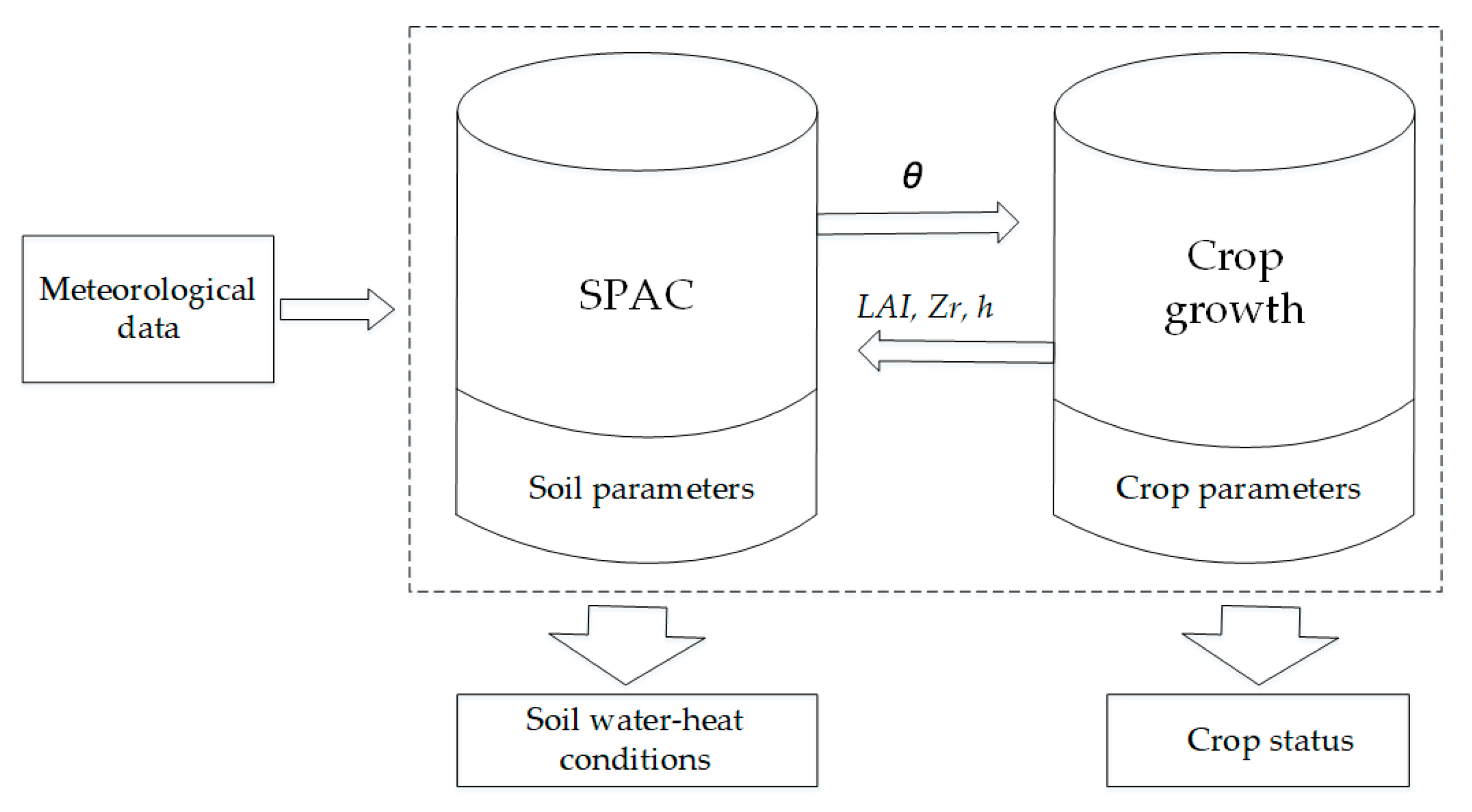
CropSPAC includes two main modules, i.e., crop module for simulating crop growth and SPAC module for simulating water-heat transfer in the SPAC system. The coupling between them is shown in Figure 1.
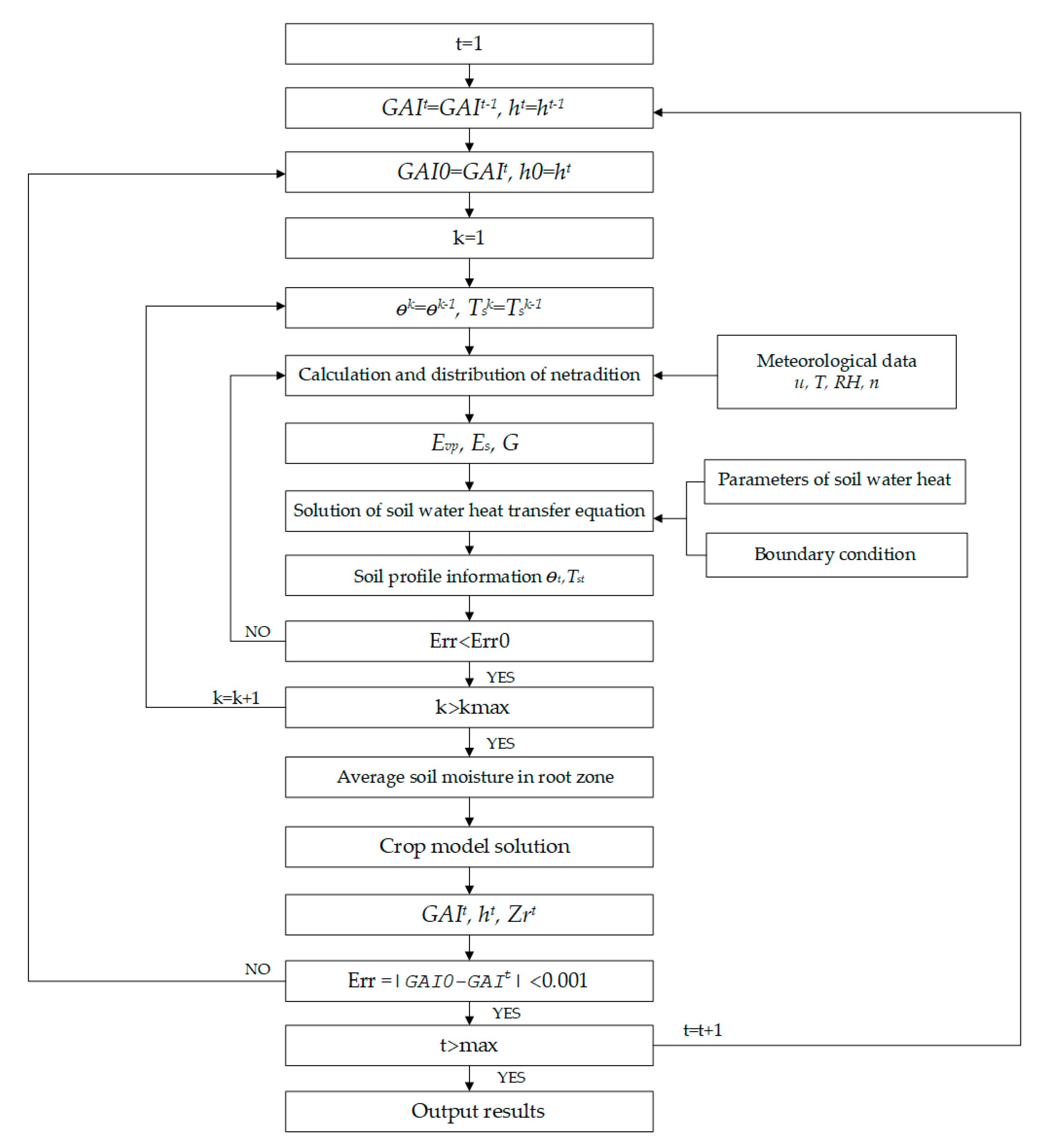
As shown in Figure 1, the output of the crop module provides input data for the SPAC module, mainly the crop information, such as LAI, root distribution, plant height, etc. The output of the SPAC module provides the input data for the crop module, mainly for the soil moisture condition, such as the averaged soil moisture content in the root zone. The calculation flowchart is illustrated in Figure 2.
Depending on the requirement of stability, explicit or implicit methods could be applied for the coupling between Crop module and SPAC module. In the implicit method, first, the crop data from previous/initial time step is put into the SPAC water–heat transfer module to obtain the corresponding predicted soil water/temperature status at the end of the time step. Then, the predicted soil water/temperature data was used in the crop module to derive the predicted crop data at the end of the time step. The predicted crop data is then used as the input for the other round of simulation till the error of predicted data in the latest two iterations is below a certain threshold. Then the simulation of a particular time step is over and the next time step starts till the process reaches the end simulation period, generally the end of the crop season. The crop module and SPAC module are described separately in the following sections.
2.2. Crop Module
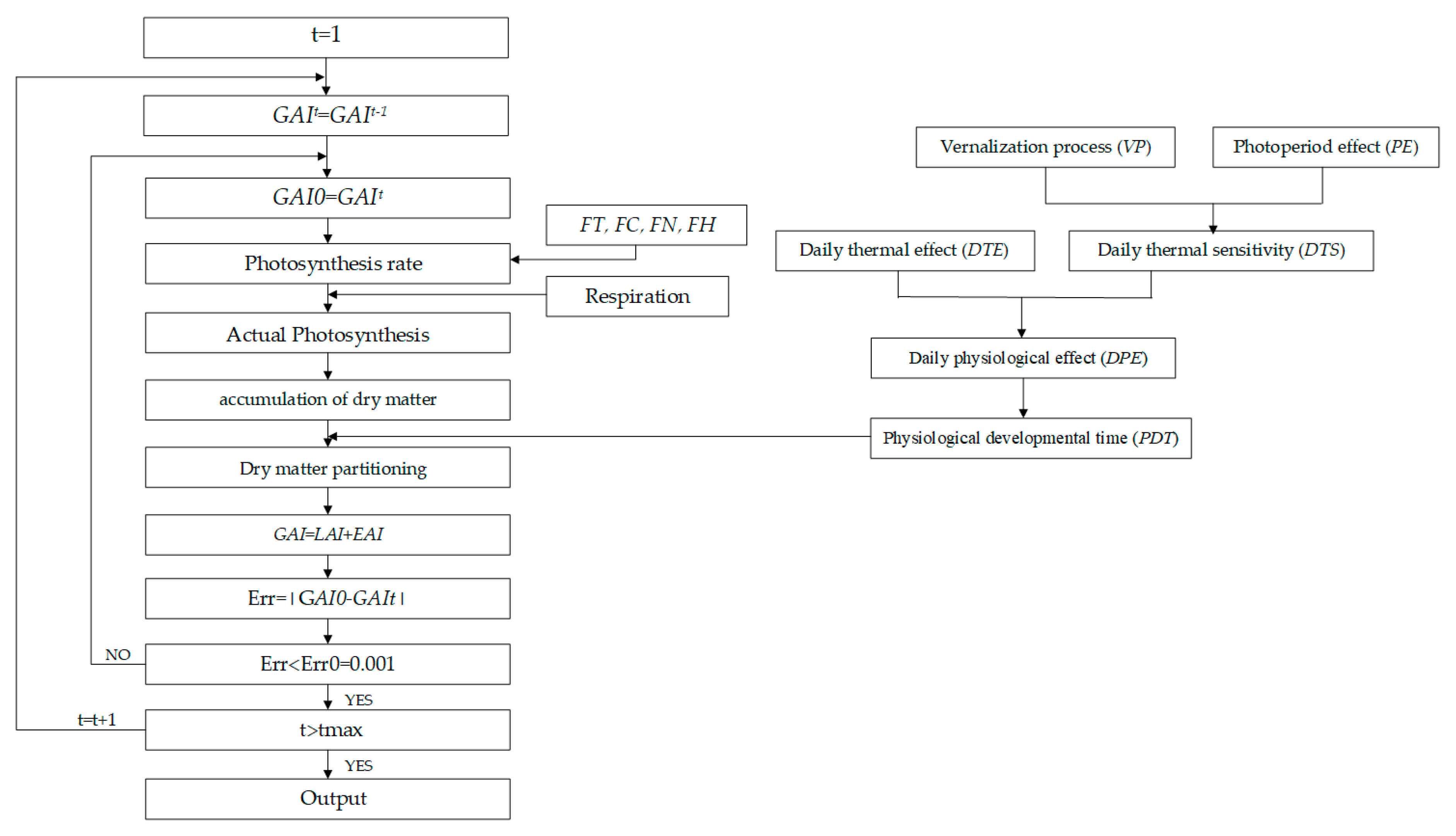
The crop module consists of three parts, i.e., simulation of crop stage development, simulation of biomass accumulation and simulation of dry biomass distribution and final yield. Here, the crop considered is winter wheat, which is a common cereal planted in North China. The calculation flowchart of the crop module is illustrated in Figure 3.
2.2.1. Simulation of Crop Stage Development
In this paper, the description of crop stage development is based on Cao et al. [27,28]. The physiological processes of stage development are generally regulated and influenced by the temperature and photoperiod. The stage development response to temperature is manifested in two forms. One is the thermal effect (TE), which the rate of stage development increases with the increase of thermal effect. The other is vernalization effect (VE), which only functioned in cold season crops such as winter wheat, generally referring to the phenomenon that plants must undergo a period of sustained low temperature then it can move from the vegetative growth stage to the reproductive stage. The sensitivity of stage developmental rate to photoperiod or daytime are called photoperiod effect (PE). For cold season crops, it is generally characterized by the longer sunshine time which will promote the crop growth rate. In addition to the temperature and light response characteristics, the crop stage development has also received species and genetic influences.
Physiological development time (PDT) is a time scale of crops in the most suitable development environment. Under any light and temperature conditions, the time for a specific crop to complete the entire growth period is essentially constant, i.e., the PDT value is basically constant, which is called the principle of constant physiological development time. Therefore, the development stage of specific genotypes crop can be predicted by [27]:
where BDF is physiological development factor, a specific genetic parameter related to the variety of the crop, the range of wheat is 0.6–1.0 according to Cao et al. [27]; the PDTt is the physiological development time without consideration of crop variety impact, which was accumulated by the daily physiological effect (DPE):
The daily physiological effect (DPE) can be represented by daily thermal effects (DTE) and daily thermal sensitive (DTS) interactions:
DTS can be calculated from [28]:
where the VP is vernalization process; PDTTS and PDTHD are PDT requirements for the terminal spikelet stage and heading stages, 10 and 27, respectively. The detail calculation methods of the DTE, VP, and PE can be found in Appendix A, and the values of some parameters above (e.g., BDF) are shown in Appendix C, Table A2.
2.2.2. Simulation of Biomass Accumulation
The formation of biomass is mainly related to the physiological and ecological processes, such as photosynthesis and respiration. The photosynthesis and biomass accumulation is based on the calculation of photosynthetic rate of single leaf, then the daily assimilation of canopy are calculated, subtracting the consumption of respiration, finally the daily net assimilation amount is calculated.
(1) Photosynthesis of crop canopy
The photosynthetic rate of single leaf is calculated as [29]:
where FG is the photosynthetic rate of leaves, kgCO2·ha−1·h−1; PLMX0 is the maximum photosynthetic rate of leaves, kgCO2·ha−1·h−1; ε is the initial utilization efficiency of absorbed light, kgCO2·ha−1·h−1·(J·m−2·s−1) −1; IL is the photosynthetically active radiation intensity at L (depth of crop canopy), J·m−2·s−1; FH is the water influence factor; FN is the nitrogen influence factor (note that the current CropSPAC model could not simulate the soil nitrogen migration, however, any nitrogen stress could be empirically indicated by this parameter); FT is the temperature influence factor; FC is the CO2 concentration influence factor. Calculation methods and details are shown in Appendix A.
Based on the single leaf photosynthesis model, the Gauss integral method [30] is used to calculate the daily photosynthesis rate of the canopy, which can greatly reduce the amount of calculation under the premise of ensuring the accuracy of calculation. The Gauss integral method divides the leaf canopy into five layers, calculates the instantaneous assimilation rate of each layer and obtains the instantaneous assimilation rate of the whole canopy. By selecting the three time points from noon to sunset, the canopy assimilation rate at three time points were calculated by weighted summation, and the daily canopy assimilation rate (FDTGA) was obtained.
(2) Biomass formation
The net assimilation rate of the population is calculated by:
where PND is net daily assimilation of population, kgCO2·hm−2·day−1; RM is consumption of maintain respiration, kgCO2·hm−2·day−1; RG is consumption of growth respiration, kgCO2·hm−2·day−1; RP is consumption of photorespiration, kgCO2·hm−2·day−1, with details shown in Appendix A.
For daily increment of dry biomass in population:
where TDRW is daily increment of dry biomass in population, kgDM·hm−2·day−1; ξ is conversion coefficients between CO2 and organic compounds.
For accumulation of dry biomass:
where WDAY is accumulation of dry biomass, kgDM·hm−2·day−1.
2.2.3. Dry Biomass Partitioning and Yield
Based on the dynamic relationship between the distribution index and the growth process [31], the distribution index of wheat organs during the growing period was established as:
where PTOP is the aboveground part distribution index, PROOT is the underground part distribution index, PLEAF is the leaf distribution index, PEAR is the ear distribution index, PSTEM is the stem and sheath distribution index, and HI is the harvest index.
In the distribution of dry biomass, the distribution index of aboveground and underground parts of the soil is also affected by the water status, and the distribution index of the leaf dry biomass is affected by both water and nitrogen.
The approximate linear relationship between winter wheat yield (YIELD) and spike weight (WEAR) was established by Cong [29]:
Based on previous study [32], the empirical relationship between LAI and leaf dry biomass quality (WLEAF) was given as:
where SLA is leaf weight per unit, general range 0.0022~0.0045 ha·kg−1 [32], and in this study it is calibrated by field data (value shown in Appendix A).
2.3. SPAC Module
In this study, the SPAC module was built on the previous work by Mao et al. [33], who established the water–heat transfer model in SPAC under soil water stress, with one canopy layer, based on soil hydrodynamics, micro-meteorology, plant physiology theory and energy balance principle. The calculation flowchart of the SPAC module is shown in Figure 4.
2.3.1. Calculation of Net Radiation and Water-Heat Transport in Crop Canopy
The formula for the net radiation of the lower cushion surface can be expressed as:
where Rn is the net radiation, W·m−2; Rg is total short-wave radiation, W·m−2; A is the land surface albedo; F is net long-wave radiation, W·m−2. The Rg, and F can be calculated by theoretical or empirical methods shown in the Appendix B [34], the value of A can be seen in Appendix C, Table A2.
Net radiation of underlying surface Rn can be divided into two parts:
where Rv is the net radiation absorbed by crop canopy, W·m−2; Rs is the net radiation absorbed by ground surface, W·m−2.
The Rs is calculated from the empirical formula summarized from field observations [35]:
where A and B is the empirical coefficient: for winter wheat, A = 0.10364, B = 0.3937; t is the local time; and SN is the time of solar noon.
Neglecting the energy consumed by photosynthesis and the amount of moisture stored in the canopy air, the canopy energy distribution can be described by [36]:
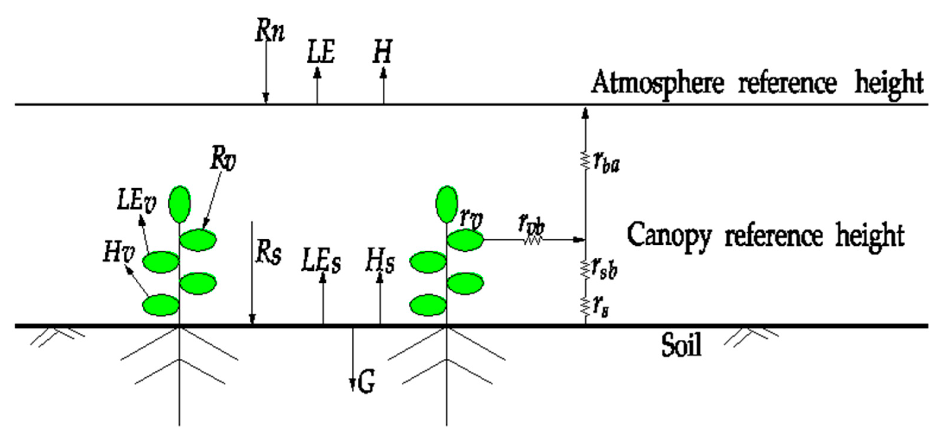
where LEv is the latent heat flux by leaf transpiration; Hv is the sensible heat flux between crop leaves and canopy air; LEs is the latent heat flux by soil surface evaporation; Hs is the sensible heat flux between soil and canopy air; G is the downward heat flux in the soil surface; H is the sensible heat flux between canopy air and the above atmosphere (usually considered at the reference height); LE is the latent heat flux between canopy air and the reference height atmosphere. The unit of the above variables is W·m−2. Schematic diagrams of energy distribution between atmospheric-ground interfaces and resistance of the hydrothermal transmission are shown in Figure 5. Detailed calculation methods are shown in Appendix B.
2.3.2. Calculation of Crop Transpiration under Water Stress in Root Zone
When the root zone is in low soil water condition, the water absorption rate by the crop root would decrease, resulting in the reduction of stomatal conductance, the decrease of leaf water potential, and the increase of stomatal resistance (rv), which induce the reduction of canopy transpiration. Plant physiologists have studied the effects of soil moisture changes on leaf water potential and stomatal resistance [37], but due to the complex mechanism involved, it is difficult to quantify directly the solve leaf water potential and stomatal resistance under soil water stress. Neglecting the water storage variation in the crop, we assume the root water uptake equals the canopy transpiration. Therefore, the response of canopy transpiration to soil water stress can be reflected by the actual root water uptake described by the soil water stress coefficient of root water uptake k(ψ). The actual transpiration of crops under the condition of water stress, Ev, can be calculated by:
where k(ψ) is the soil water stress coefficient of root layer, depends on the distribution of root density and the corresponding function of water stress, which is derived in next section and shown in Equation (34); Evp is the potential transpiration without water stress in root zone.
Hence the latent heat flux between crop leaves and canopy air (LEv, see Equation (A42)) can be replaced by Equation (26):
where rv0 is the canopy total stomatal resistance under no soil water stress, s·m−1.
2.3.3. Water and Heat Transfer in Soil with Root Water Uptake
Richard’s equation under root water absorption conditions and heat conduction equation is used to describe soil water–heat transfer:
where θ is the soil water content, cm3·cm−3; T is the soil temperature, °C; t is the time, s; z is the depth from the surface, m; Dw is the coefficient of soil water diffusion, m2·s−1; Dwh are the diffusion coefficients of temperature gradients to water flow, m2·s−1·°C−1; Kw is soil water conductivity, m·s−1; Cv is soil volumetric heat capacity, J·m−2·°C−1; Kh is the soil thermal conductivity, J· s−1·°C−1; s(z,t) is the distribution function of the actual water uptake rate of roots, m3·m−3·s−1; Sh is the heat source sink term, J·m−2·°C−1, generally negligible.
There are three types of root density distribution function commonly used in the research, including the evenly distribution, the linear variation distribution with root depth, and the exponential distribution with root depth. Here we used the linear variation function, assuming the ratio of upper part root density to lower part root density is 0.7/0.3, which is in accordance with previous research [38].
We assume the maximum potential transpiration Evp, which is not limited by soil water stress, equal to the potential total root water uptake rate, i.e., the integration of potential root water uptake rate along the entire root zone considering the root density distribution. The actual root water uptake rate s(z, t) is equal to the potential root water uptake rate s0(z, t) multiplied by water stress response function α (ψ, π) [39]:
where ξ’(z, t) is relative root density function; ξ(z, t) is root density function; ψ(z), π(z) is soil matric potential and solute potential at the depth z below ground surface respectively, P is an empirical constant, ψ50 is the specific soil water potential, when Evp decreases by 50%(ψ50 ≈ −0.43 MPa); Zr is the depth of the root zone.
Through Equations (32)–(34), the expressions of the root water uptake rate distribution, the crop transpiration and the corresponding soil water stress coefficient of root water uptake at a certain time can be derived as:
For the two non-linear partial differential equations (see Equation (27)), they are high non-linear, could be solved by implicit finite difference methods in order to reduce the numerical oscillations. Iterations between the above ground and soil processes might be required considering the calculation stability.
3. Experiment and Model Input
3.1. Study Area and Experiment
The experiment data were collected from a farmland planted with winter wheat (Triticum aestivum L.) in Yongledian Experiment Station, Beijing, China from October 1998 to June 1999. The experiment station is located at 116°40′ E and 39°47′ N with an average elevation of 12 m above sea-level. The average annual temperature in the region is about 11.5 °C. The average annual rainfall is about 570 mm, and most of the rain falls in the period from June to August. The soil is sandy loam with the bulk density of 1.4 g·cm−3, and the depth of water table is mostly larger than 5 m in this area.
Daily meteorological data were recorded by a weather station at the experimental site, including solar radiation, sunshine hours, air temperature, humidity, atmospheric pressure, wind speed, and precipitation. Soil water content was measured with neutron hydroprobe and tensiometer (503DR, Campbell Pacific Nuclear Corp., Martinez, San Francisco, USA), which were measured every 20 cm soil layer till the depth of 100 cm. For the soil temperature measurement, thermistors manufactured by the Chinese Academy of Agriculture Sciences were installed and were monitored in soil depth of 10 cm, 20 cm, 30 cm, 40 cm, 60 cm, 80 cm, and 100 cm. Crop characteristics, e.g., crop height, was measured with a meter ruler, and leaf area index was calculated as the product of plant density and average green leaf area of individual plant, with the leaf area estimated from the product of length, maximum width and leaf form factor (0.83 for winter wheat) [40]. Dry biomass was calculated from the product of plant density and average dry weight of individual plant, with the dry weight determined after drying for 24 h at 80 °C in a fan-forced convection oven.
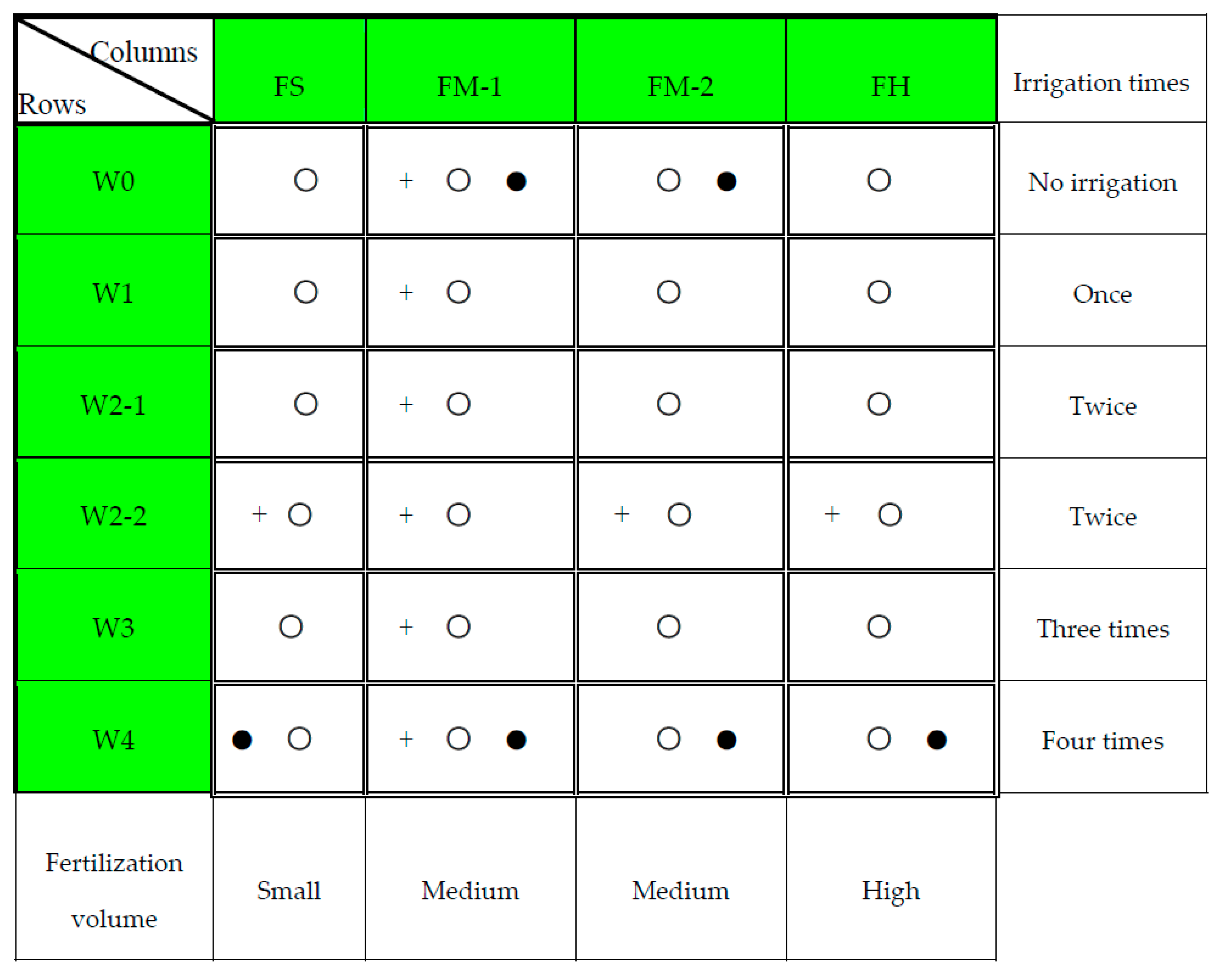
The experiment field was divided into 24 experiment plots, with the area of each plot 50 m2 (5 m × 10 m), as shown in Figure 6. It includes six rows for five irrigation treatments (two rows for W2 treatment), and four columns for three fertilization treatments (two columns for medium level fertilization treatment). Since only column FM-1 has crop growth index monitoring, the medium fertilization with five levels of water treatments were used for model calibration and validation. In those treatments, the level of fertilization is the same, which was reflected in the factor FN (e.g., FN is assumed to be 0.95) in CropSPAC. The details of fertilization volume, irrigation volume, and time were shown in Table 1.
Usually, the winter wheat grows in dry seasons from October to early June of the next year. During the soil frozen period from late November to next February, wheat grows very slowly or even stops for about 100 days. Note that our current model for soil water–heat transfer does not include the soil water freezing and thawing period. Under such condition, more complex mechanism should be involved and could only be solved by some specific soil water–heat transfer model, like THAW [41]. Since our model has difficulty to simulate the soil frozen period, we set the CropSPAC model to start simulation on March 20, and assume the initial value of the crop information at this time based on empirical experience (the initial value of the crop information can be found in Table 2 in Section 3.2).
3.2. Model Input
The input for the simulation includes meteorological conditions, crop parameters, initial crop physiological index, soil water and thermal characteristics parameters, and initial and boundary conditions of soil temperature and moisture.
Meteorological parameters of the model input include daily average wind speed, sunshine hours, daily maximum and minimum temperature, daily maximum and minimum water pressure, irrigation and rainfall, etc., which were provided by weather station. The crop parameters related with winter wheat were illustrated in the Appendix C, Table A2, as mentioned in Section 2.1. The simulation period starts from March 20. The initial crop physiological index on this date was determined based on the empirical experience with calibration, as shown in Table 2.
The relationships among soil water content, matric potential and hydraulic conductivity can be described by van Genuchten-Mualem (VGM) model [42,43], and the related soil hydraulic parameters for the station were calibrated with field data and shown in Table 3. Soil thermal parameters, Kh and Cv, mainly vary with the soil water content, can be described by Johansen model [44].
For the soil water and heat movement, the equations were solved numerically by finite difference method. The time step usually was in hourly level which could be automatically adjusted according to the numerical stability. Note that the weather information and the other boundary conditions were usually obtained on daily bases, which needed to be refined accordingly to fit the requirement of this numerical simulation, e.g., for the hourly temperature, it is obtained based on the sine function and the daily monitored maximum and minimum temperature. For the more detailed temperature, it is obtained by linear interpolation based on the hourly temperatures. At the beginning of the simulation, the initial soil moisture and temperature along the soil profile were given by the measured values.
When there was no precipitation and irrigation, the upper boundary of soil moisture movement was the evaporation boundary, and the evaporation rate Es was calculated based on the above ground water–heat transfer and energy participation. When there was irrigation or precipitation, the upper boundary condition was switched to the Dirichlet boundary. The upper boundary of soil temperature was Neumann boundary, with the flux, i.e., the downward heat flux to the soil, obtained from the above ground calculations. The lower boundaries of soil water and soil temperature were set to be the Dirichlet boundary, based on the measured values.
4. Simulation Results
The established CropSPAC model was manually calibrated and validated by field data in Yongledian. W0, W2, and W4 treatments were used for calibration, then the W1 and W3 treatments were used for validation to the calibrated model.
4.1. Soil Water Content
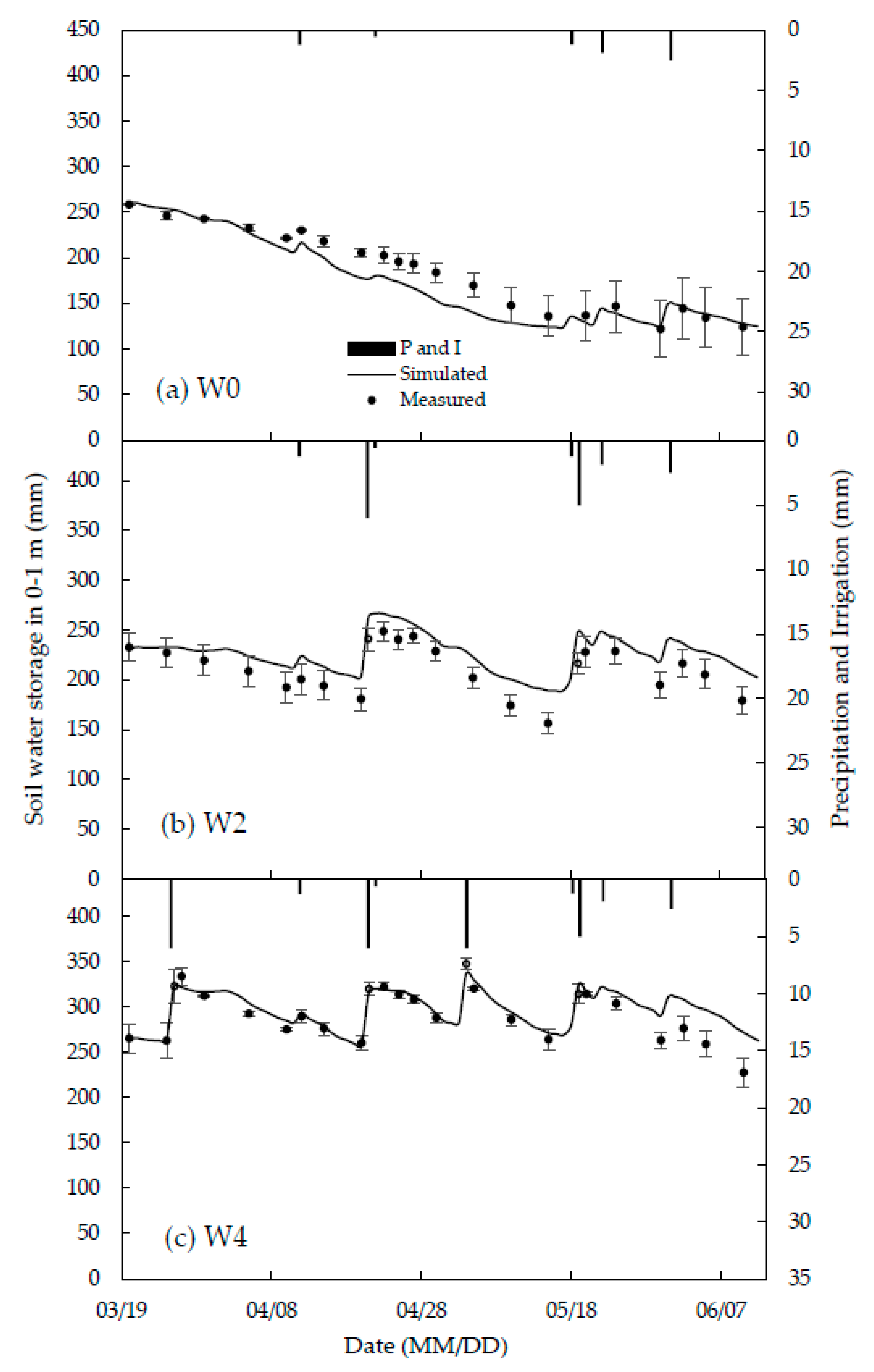
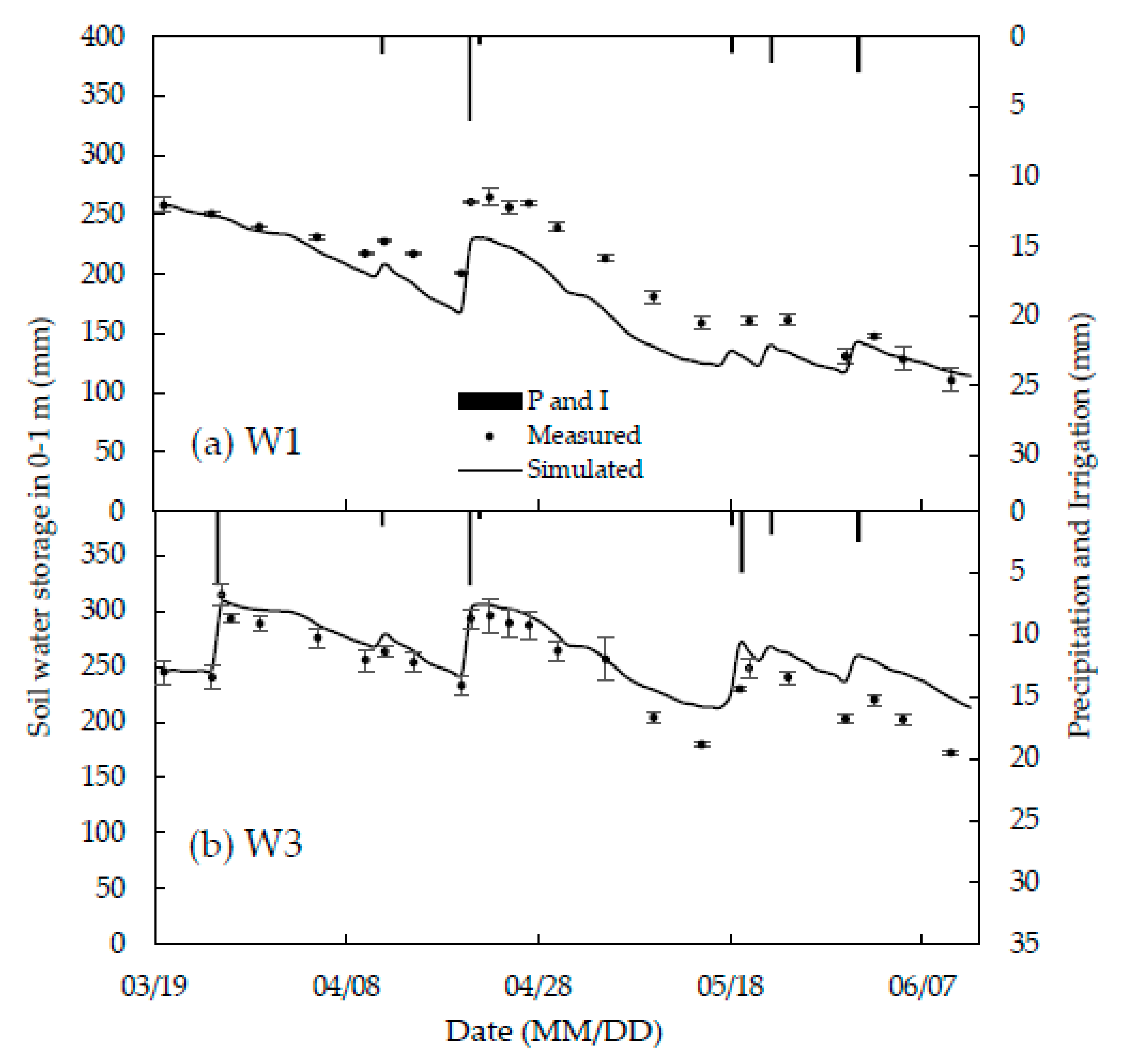
The calibration and validation results of soil water storage in the 0–1 m soil layer are shown in Figure 7 and Figure 8. All the treatments show that the soil water storage in the root zone was affected strongly by the surface irrigation/precipitation and the evapotranspiration process. After each event of irrigation or large rainfall, the soil moisture increased sharply (such as, on March 26, April 21, May 4, and May 9 in W4), and then decreased gradually due to the spring wheat roots water uptake, soil surface evaporation and deep percolation, similar to the previous studies, e.g., Shang et al. [45]. In the early stage of crop growth, the soil water storage decreased more slowly because of the less root water uptake and small evapotranspiration in the early stage of crop growth. In the middle and late growth stages, with the increase of LAI and the increase of potential atmospheric evaporation, the evapotranspiration of crops increased, resulting in the rapid decline of soil water storage. The R2 in W0, W2, W4, W1, and W3 is 0.90, 0.90, 0.79, 0.88, and 0.91, and is RMSE 17.24 mm, 20.47 mm, 12.88 mm, 27.65 mm, and 22.35 mm, respectively.
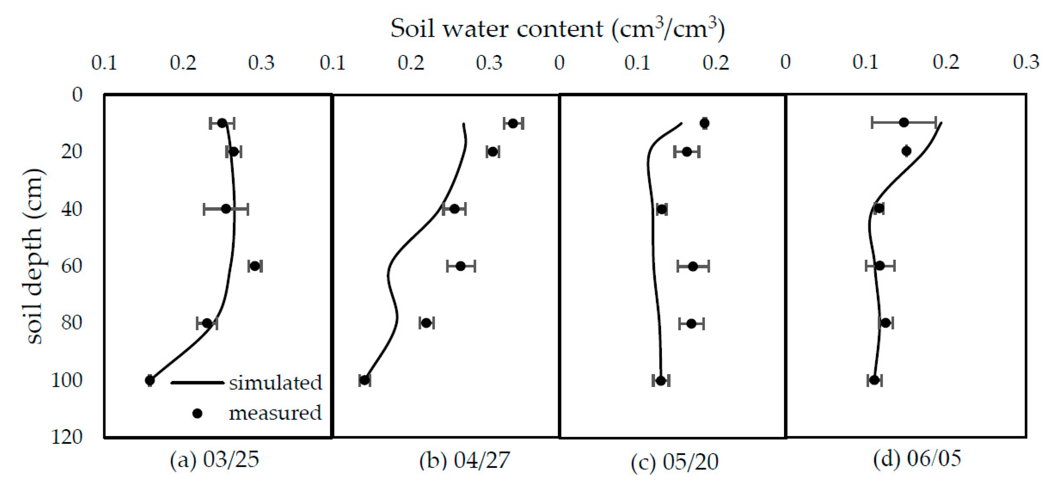
Comparison between simulated and measured soil water content of different soil layer are put in Figure 9 and Figure 10 (only W4 and W1 was shown in this article due to the limits of length). Most of the soil profiles simulation results agreed well with the experiment, with the R2 on March 25, April 27, May 20, and June 2 in W4 of 0.92, 0.24, 0.74, 0.61, March 25, April 27, May 20, and June 5 in W1 0.89, 0.78, 0.23, 0.91, and the corresponding RMSE of 0.01, 0.03, 0.02, 0.03, 0.01, 0.05, 0.03, and 0.02, respectively.
Although the trend between observation and simulation are similar, there was still some error between the two sets of data, especially in the late stage where the simulated results showed higher soil water storage than the observed data, e.g., Figure 7b,c, and in some soil profiles simulation results, e.g., Figure 9d and Figure 10b. One of the reason for simulated deviation should be the lack of local crop parameter information which requires further study to determine them more accurately. The other should be caused by the soil heterogeneity. In general, the simulated soil water content values were in reasonable agreement with the measured value under the different water treatments.
4.2. Soil Temperature
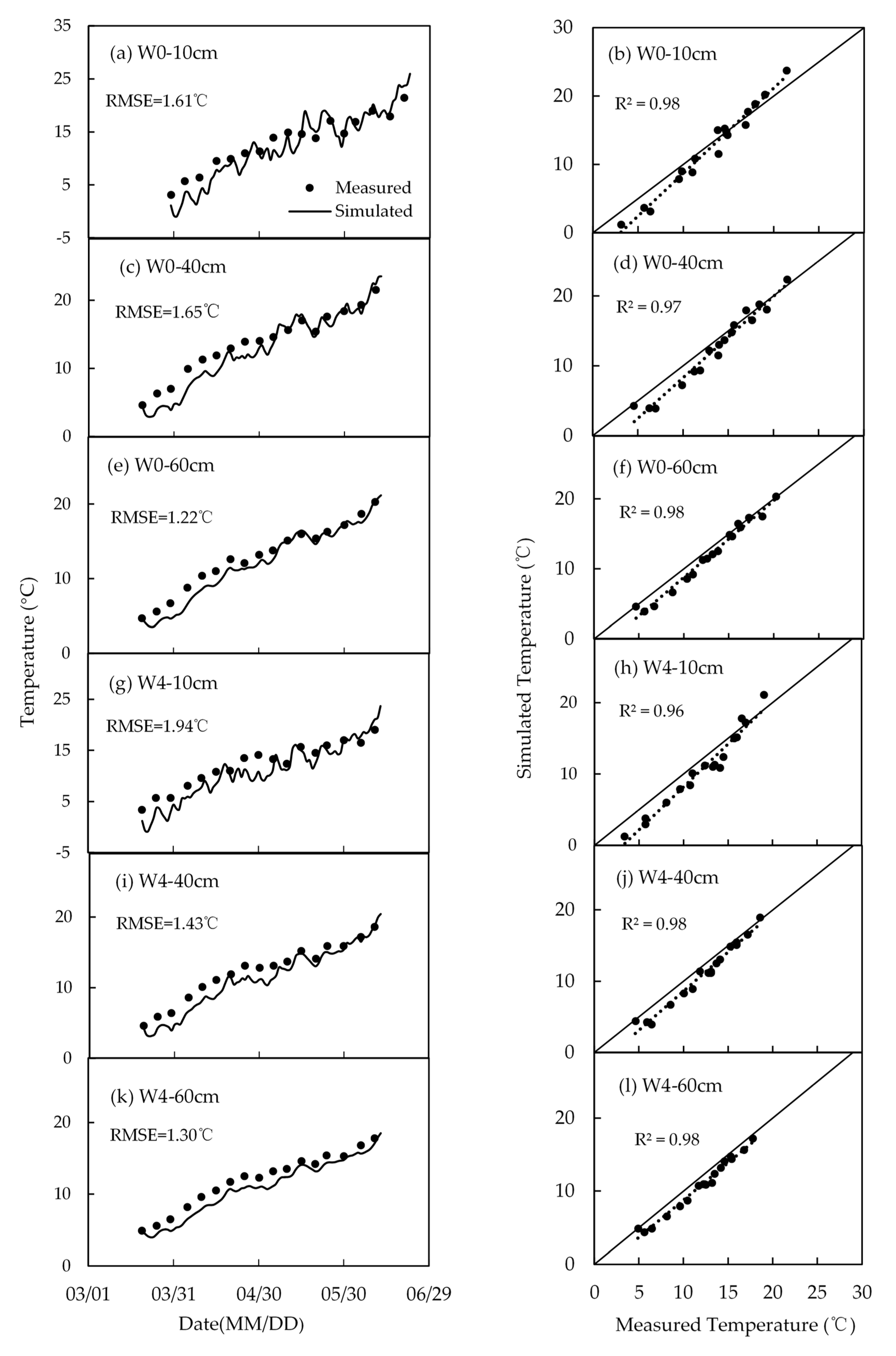
The simulated and measured soil temperature at different soil layers were shown in Figure 11. (note that only W0 and W4 have measured temperature data). The net radiation absorbed by the ground surface, Rs, was mainly consumed by the soil latent heat, sensible heat, and the downward heat flux. In this simulation period, with increase in atmospheric temperature and surface downward heat flux (G), the soil temperature in each layer showed a gradually increasing trend. Additionally, soil temperature fluctuated more greatly in upper soil layers, because the upper soil was more exposed to atmospheric temperature and surface radiation.
The simulated results showed good agreement with the measured values. The range of R2 varied between 0.96 and 0.98, and RMSE ranges from 1.22 °C to 1.94 °C. However, it seems the simulated results systematically underestimated soil temperature generally in the early crop stage. The reason may be, (1) according to the observed air temperature, there is a large drop on March 22. It is captured in the simulation with the soil temperature dropped accordingly, especially in the near surface layers. However, strangely the observed data did not show this drop, possibly because some artificial measure had been taken to keep the soil temperature which was unable to be captured in our model; and (2) due to the uncertainty of local crop parameters, the simulated LAI tended to be higher in the early crop stage. Thus, the larger canopy meant larger interception of radiation and less radiation absorbed by the soil surface. Therefore, the simulated soil temperature tended to be small in the observed data in the early crop stage. With more work on the accuracy of crop data and the detailed investigation of agriculture management, the simulation performance was able to be improved in future research.
4.3. Leaf Area Index
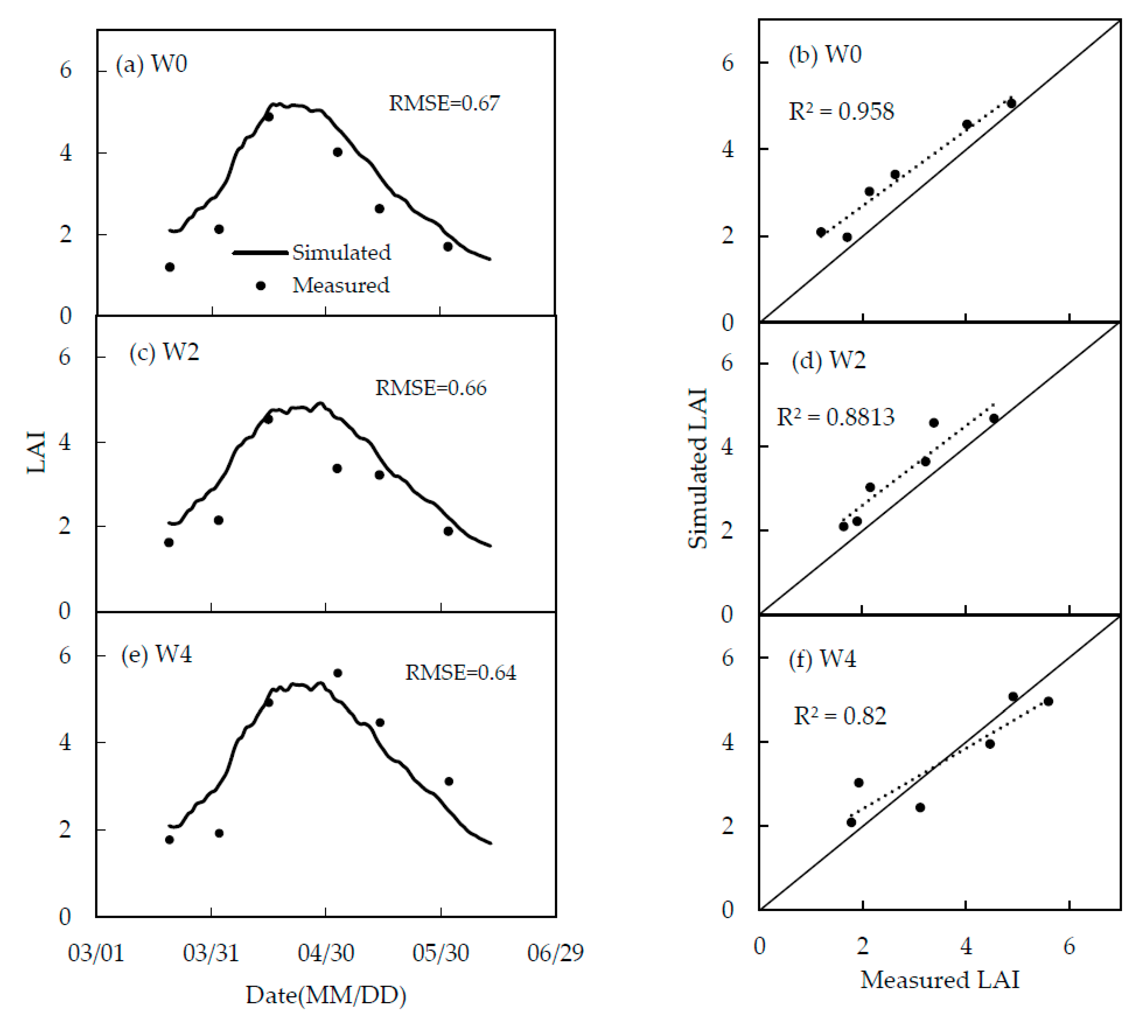
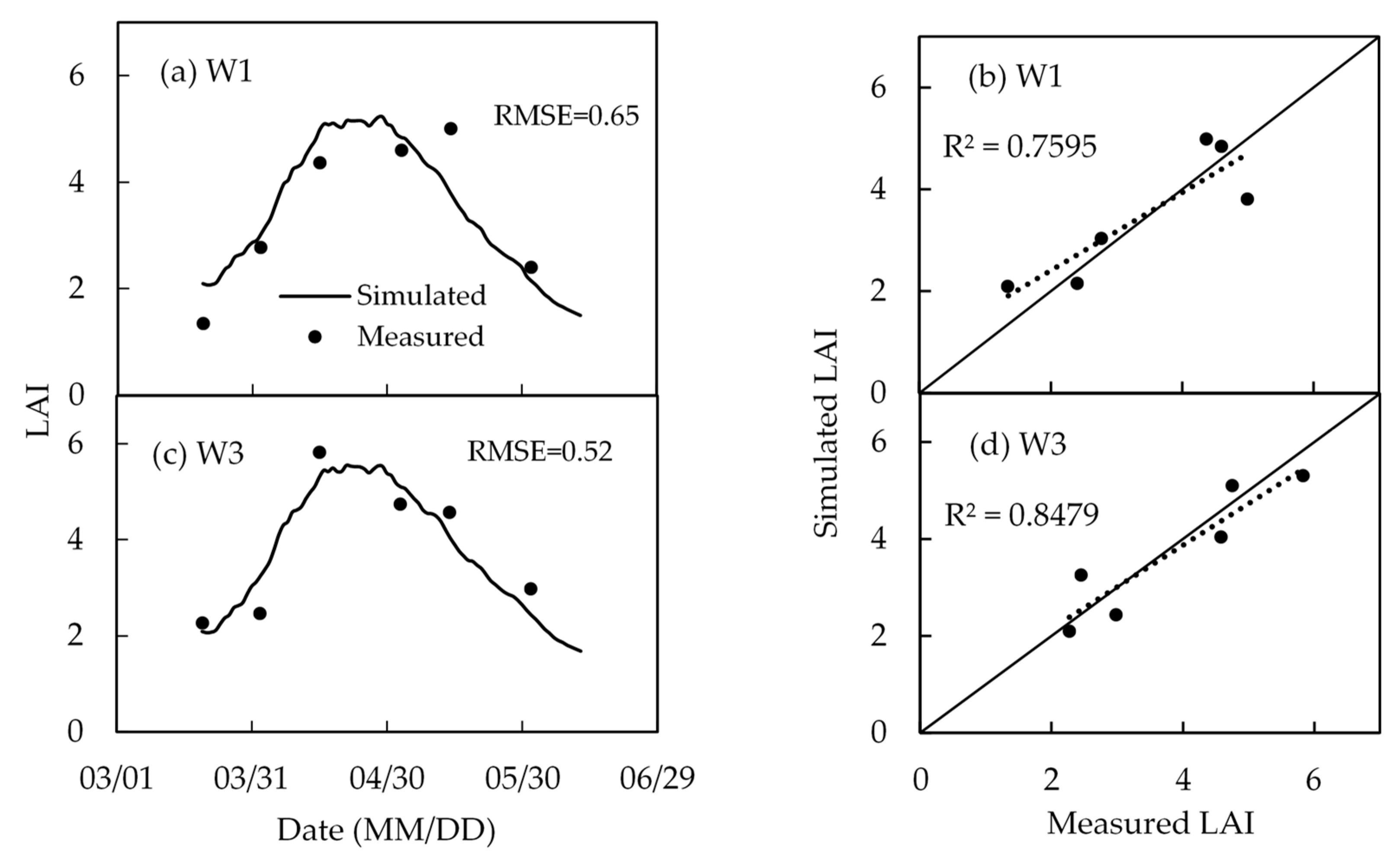
Figure 12 and Figure 13 present the comparison between simulated and measured LAI results, which showed the dynamic changes of LAI of winter wheat from turning green to maturity stage. Simulated and measured values showed similar trends, with the R2 ranging between 0.76 to 0.96, RMSE between 0.52 and 0.67. From early March when winter wheat turned green, leaf area and dry biomass gradually increased with the increase of air temperature. When winter wheat entered the grain filling stage, the LAI reached the maximum value. Then the leaves got senescent and LAI declined, and the dry biomass accumulated by the plant transfers from the organs to the ear. The peak and time when the LAI reached this maximum value in the three treatments were different as shown in Figure 11. For example, in W4 treatment with the adequate irrigation water supply, it is in the beginning of May that LAI reached its peak value of 5.6, while in W2 and W0 treatments the time is in early April, with the peak values also smaller at between 4 and 5. This illustrated that deficit irrigation limited the growth of crop and the extension of the foliage, and led to the crop early mature. This is also a kind of physiological protection measures for plants in the shortage of water supply, mature in advance to avoid large-scale production loss, as demonstrated by other research [46,47].
However, the model overestimated the value of LAI in early stage of crop growth. One possible reason is that the LAI in the model was calculated by the relationship between the LAI and the dry biomass of leaf, and the simulation of dry biomass by the model was slightly larger in early stage (seen in Figure 13 and Figure 14), so that the simulated value of the LAI also appeared to be large in the previous period. The coefficient between LAI and leaf dry biomass was empirical and may differ from this specific local crop, thus contributing to the inaccurate simulation value. The gap between measured and simulated value can also be induced by the measurement errors. In general, the gradient of LAI between different water treatments is obvious, and the model fitting results were basically acceptable.
4.4. Biomass and Yield
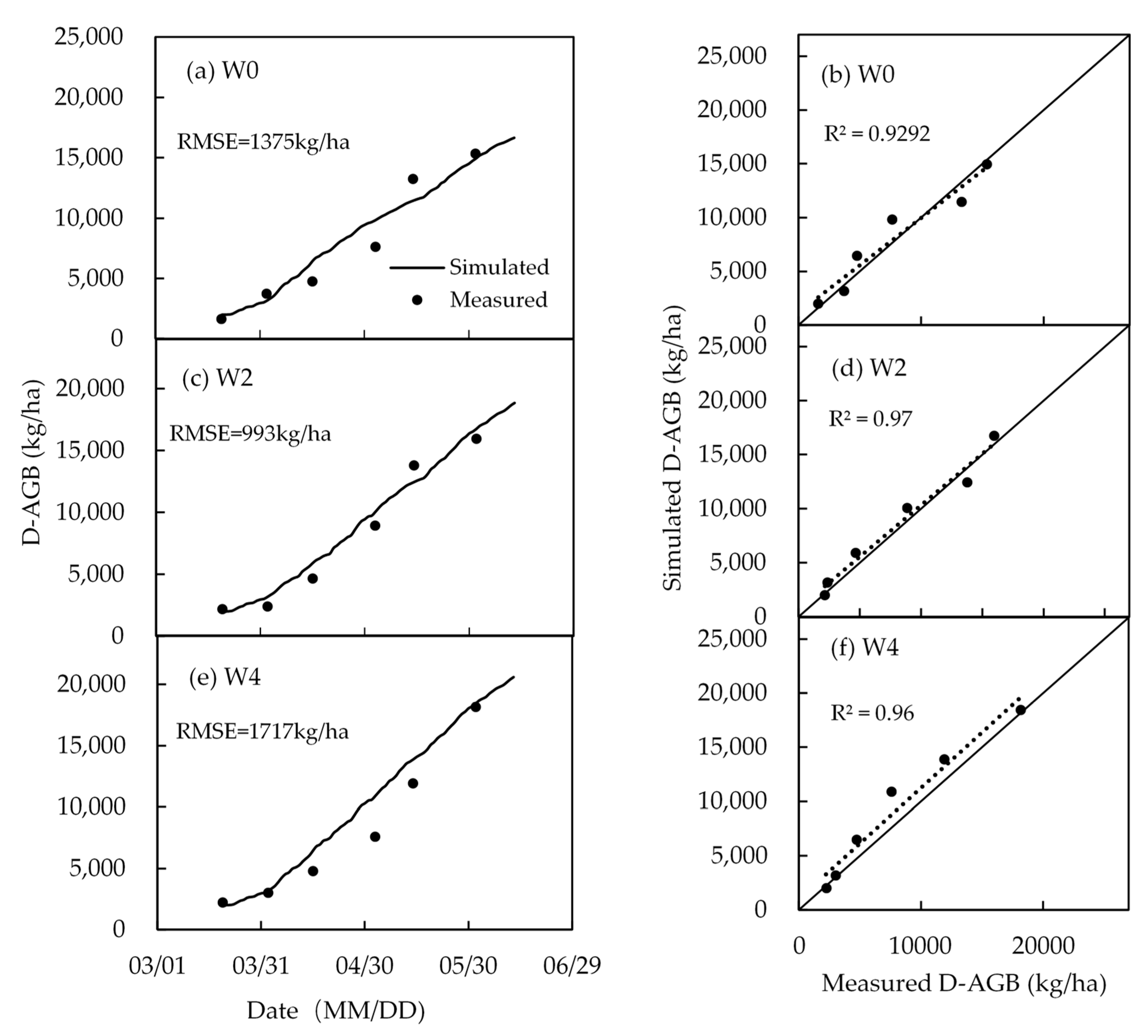
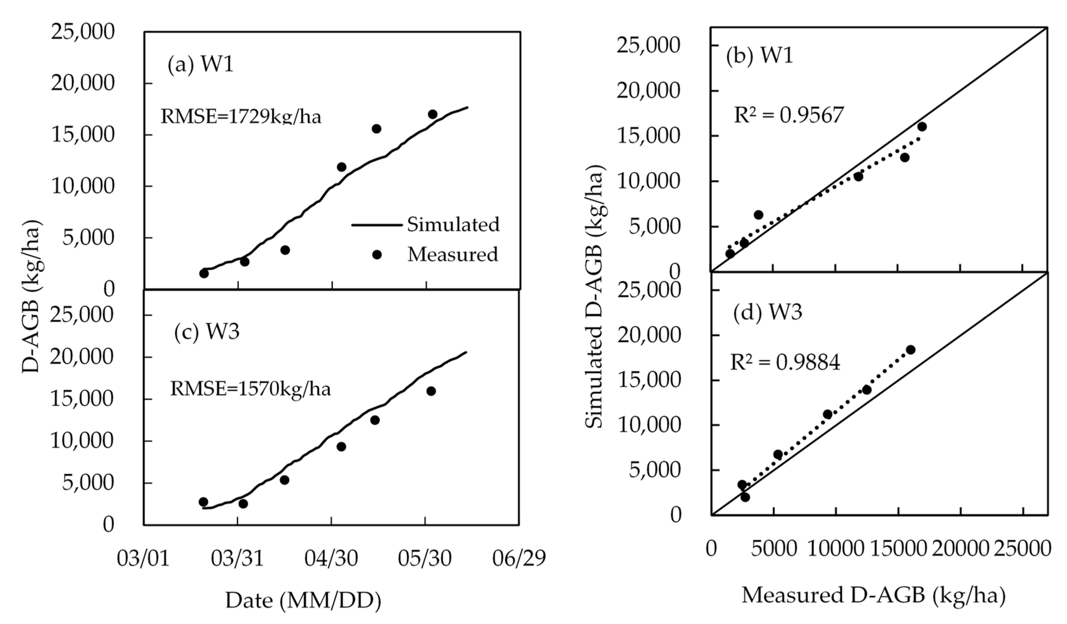
Figure 14 and Figure 15 show the results between the measured and simulated dry aboveground biomass (D-AGB) and Table 4 shows the measured and simulated yields. With the growth of spring wheat, the dry aboveground biomass gradually increased. The CropSPAC model simulated the accumulation of D-AGBin spring wheat with the R2 varied from 0.93 to 0.99 and RMSE from 993 kg/ha to 1729 kg/ha in different treatments. The increase in irrigation contributed to the accumulation of dry biomass. The reduction in water directly led to a reduction in dry biomass accumulation and then affected the final yield. As a whole, the simulation of the CropSPAC on the accumulation of winter wheat biomass and the final yield is reliable.
5. Discussion on the Coupling Effect of Model
5.1. Comparison between CropSPAC and the Detached Crop Module
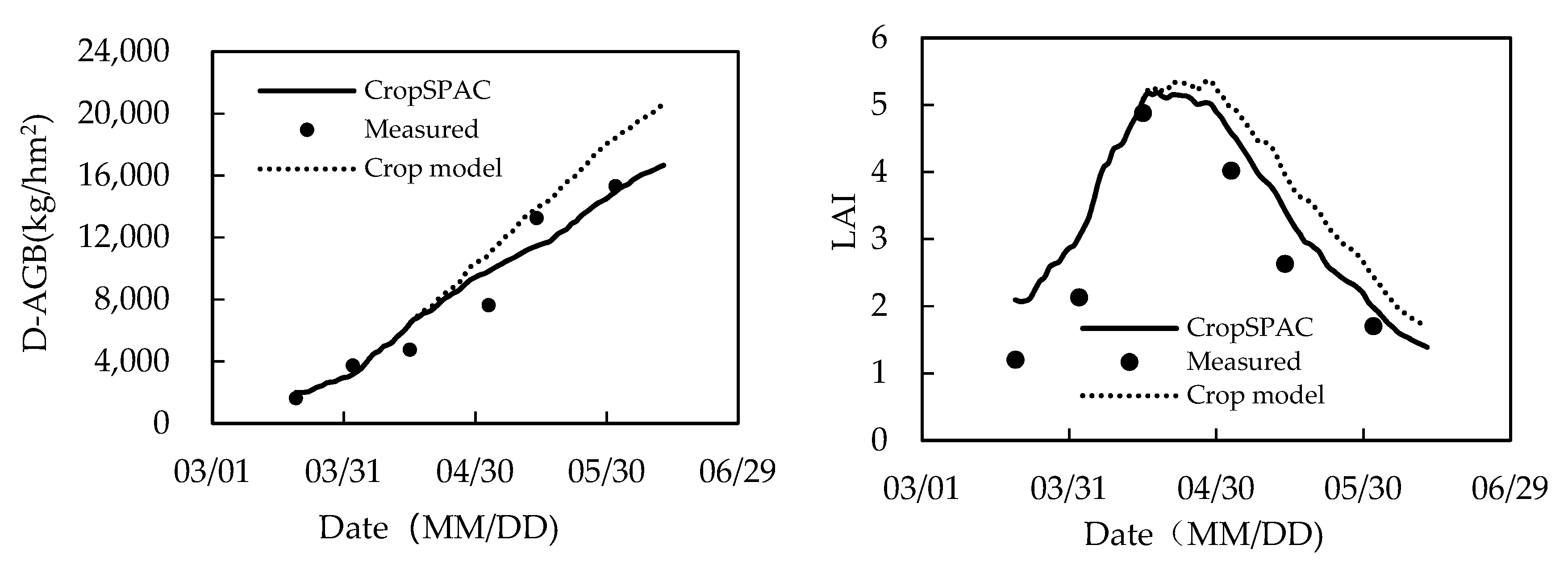
To illustrate the advantage of CropSPAC compared with the crop growth model without considering the influence of SPAC water–heat transfer, the crop module was detached from CropSPAC for simulation of crop growth. Since the soil moisture was regarded as specified input, the detached crop module may not transfer soil water deficit information to crop growth under deficit irrigation, therefore the crop growth indexes such as LAI and dry aboveground biomass could not dynamically respond to soil moisture changes, resulting in higher simulated values as shown in Figure 16 for simulating W0 treatment. While in CropSPAC the crop growth status could be directly influenced by the updated soil moisture status, making the coupled model, CropSPAC, more accurate for simulating crop growth under water deficit conditions.
5.2. Comparison between CropSPAC and SPAC
CropSPAC model could also outcompete the detached SPAC module for water–heat transfer that ignores the influence of crop growth. SPAC model only accounts for the water–heat transfer from soils to plants, and then to atmosphere, while the crop growth and canopy development is not taken into account. Therefore the detached module of SPAC is inadequate because there is a close relationship between crop growth and water–heat transfer, where the leaf extension and root development of crops will actively affect energy distribution in the canopy and root water absorption.
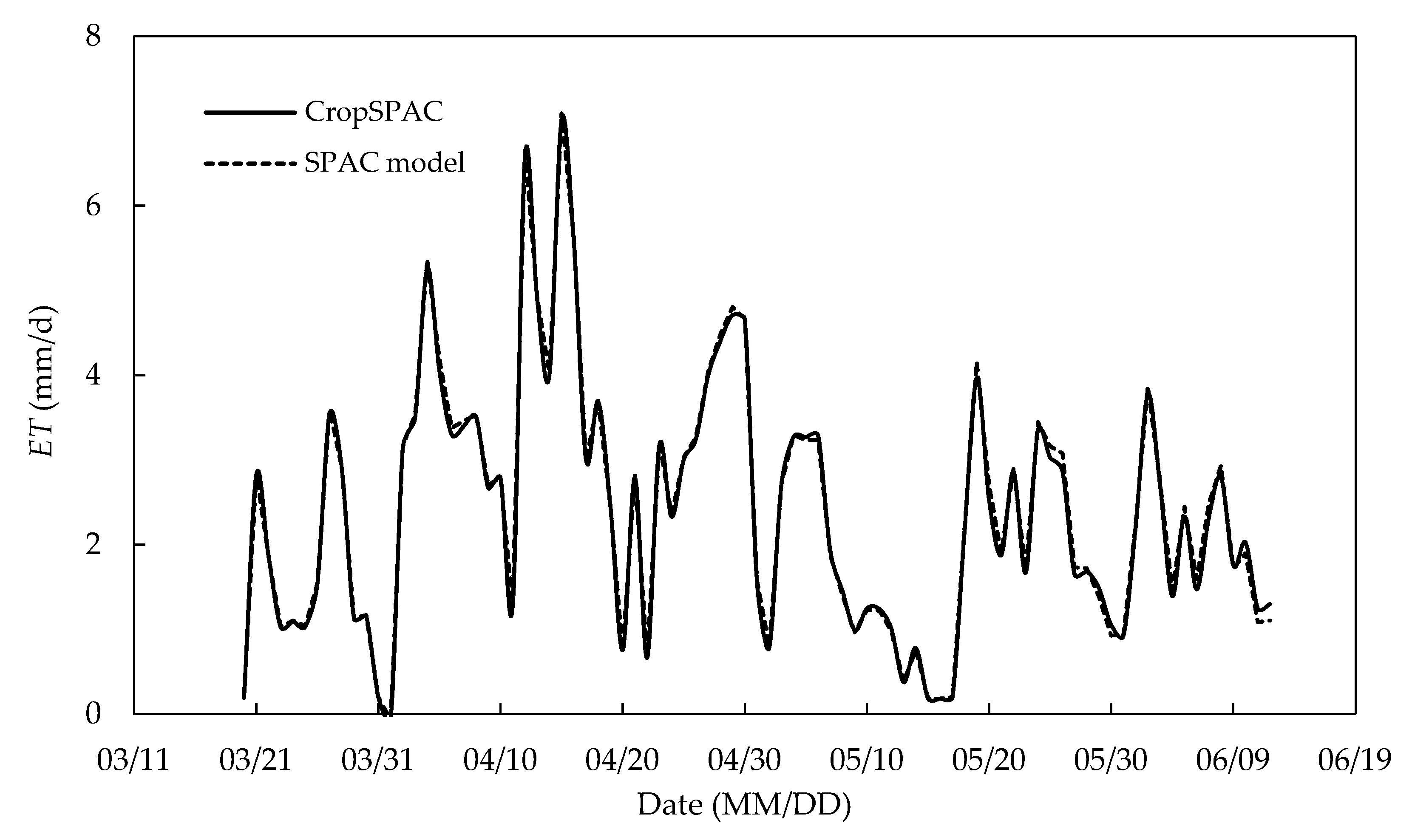
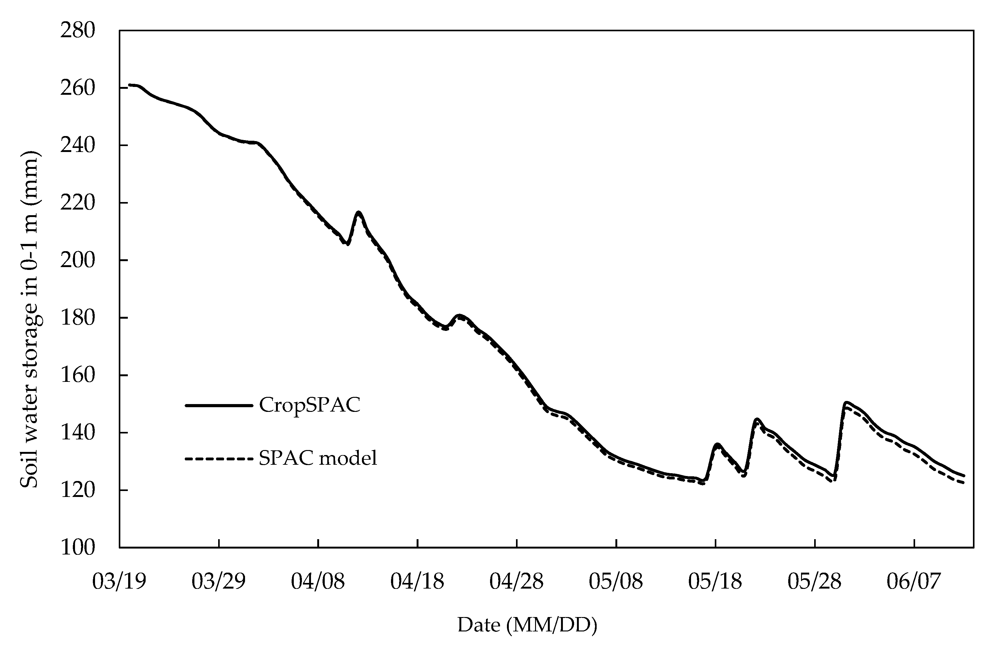
The simulation results of the CropSPAC model and the SPAC hydrothermal transport model under water deficit conditions (W0 treatment) were, thus, compared and analysed (see Figure 17 and Figure 18). The crop evapotranspiration simulated by the coupled CropSPAC model was less than the SPAC module, while the simulated value of soil water storage in 0–1 m was larger than the SPAC module. It means under deficit irrigation, the crop module of the CropSPAC model could predict the reduction of the LAI of the crop and feed it back to the SPAC module. While in the detached SPAC model, crop information, such as LAI, plant height, root growth, etc., were specified as input data, which does not change when water deficit occurs. Therefore, in case the actual LAI decreased, the detached SPAC module still used the given value (this value generally is greater than the actual LAI), which led to the larger crop transpiration in detached SPAC module. Accordingly, the root water absorption was also greater than the actual value, and then the soil water storage capacity was less than the actual value. Therefore, CropSPAC model that takes into account the dynamic changes in crop growth can better describe and simulate the dynamic changes of soil moisture and evapotranspiration under water stress.
6. Conclusions and Future Work
In this study, we present a new coupled model (CropSPAC) in which the mechanism of interactions between SPAC water–heat transfer and crop growth is considered. Winter wheat, as one of the most important food crops in North China, is affected directly by the soil hydrothermal conditions, and meteorological conditions, such as solar radiation, air temperature, air humidity, wind speed, precipitation, etc., during its growth season and yield formation. Additionally, the crop growth can also affect the water–heat transfer in SPAC. Thus, the CropSPAC model not only reflects the effect of soil moisture on the growth and yield of winter wheat, but also the effect of crop growth on the water–heat transfer process of SPAC.
The model was validated by using field measurement data from the Yongledian Experimental Station (1998–1999) in Beijing. The simulated soil water content, soil temperature at different depths, evapotranspiration, and crop growth index were in reasonable agreement with the measured values. The CropSPAC model can simulate the water–heat transfer process in the soil, and the process of crop growth more accurately, reliably, and effectively compared with the detached crop module and SPAC module. CropSPAC can be used for scenario analysis, whereby varying the irrigation times and irrigation volumes, the best combination of yield, economic benefit, and water use efficiency could be selected. Therefore, the model can provide decision support and a theoretical basis for the water-saving and yield-increasing of winter wheat and evaluation of irrigation water use efficiency. For this purpose, an optimization procedure would be designed for this model in further research.
Note that the current CropSPAC model contains only one crop, i.e., winter wheat. With the deepening of research, various types of crops, such as maize, rice, soybeans, etc., should be taken into account and the model should be validated on more climatic and geographical conditions, e.g,, maize, as a C4 crop, is different from C3 crops (e.g., wheat) in phenology development, photosynthesis, and biomass partitioning from wheat (C3 crop) and need to be considered in the future version of CropSPAC. Furthermore, with the advantage of considering both water and heat transfer, as well as energy partitions in the canopy, the coupled model can be potentially used under field mulching conditions, which is widely applied in North China and should be considered in future study.
Author Contributions
Conceptualization: X.M.; formal analysis: W.Y., X.M., and J.Y.; investigation: J.Y.; methodology: W.Y. and M.J.; supervision: X.M.; writing—original draft: W.Y.; writing—review and editing: A.J.A.
Funding
This research was funded by the National Key Research and Development Program (2016YFC040106-3) and the Chinese National Natural Science Fund (91425302, 51679234).
Acknowledgments
The valuable comments from editors and anonymous reviewers are greatly appreciated.
Conflicts of Interest
The authors declare no conflict of interest.
Appendix A. Supplementary Description of the Variable Formula in the Crop Module
1. The Calculation of Stage Development Variables
(1) Thermal Effect
The TE can be described by the sinusoidal exponential equation, as shown below [27]:
where TEi is the hour thermal effect; DTE is the daily thermal effect; Ti is the hour temperature of air, °C, i = 1, 2, …, 24; Tb is the base temperature of crop growth, °C; T0 is the optimum temperature of crop growth, °C; Tm is the maximum temperature of crop growth, °C; ts is temperature sensitivity, which is genetically determined by genetic parameters. For winter wheat, the values of Tb, T0, and Tm are shown in Table A1.

Table A1.
The parameters of thermal effect for winter wheat.
| Tb (°C) | T0 (°C) | Tm (°C) | |
|---|---|---|---|
| Emergence date to double ridge date | 0 | 20 | 32 |
| Double ridge date to heading date | 3.3 | 22 | 32 |
| Heading date to maturity | 8 | 25 | 35 |
(2) Vernalization Effect
Vernalization is the induction of the crop flowering process by exposure to the prolonged low temperature [48], which can also prevent the damage of the cold-sensitive flowering meristem during the winter [49]. The calculation of the VE in wheat is:
where VEi is the hour vernalization effect; Tbv is the minimum vernalization temperature, −1 °C; Tol is the lower limit value of the optimum vernalization temperature range, 1 °C; Tou is the upper limit value of the optimum vernalization temperature range, °C; Tmv is the highest vernalization temperature, °C; vef is the vernalization effect factor. Tou, Tmv, and vef can be calculated as:
where PVT is the physiological vernalization time, the value shown in Appendix C. When the temperature is higher than 27 °C, and the number of vernalization days does not exceed 1/3 of the physiological vernalization time, the wheat will devernalize. The devernalization effect (VED) increases with increasing temperature, which can be written as:
Daily vernalization effect (DVE) is affected by the effects of VE, and VED:
Therefore, the vernalization days (VD) on t day can be expressed as:
The vernalization process (VP) is expressed by the ratio of VD to PVT. When VD is equal to PVT or VP reaches 1, the vernalization is considered to be over:
(3) Photoperiod Effect
The PE is the sensitivity of stage developmental rate to photoperiod or daytime, mainly related to crop varieties and the length of theoretical sunshine hours and can be described by [50]:
where PS is the photoperiod sensitivity (value shown in Appesdix C); and DL is the theoretical sunshine duration, h.
2. The calculation of absorbed light
The calculation of IL (photosynthetically active radiation intensity at L depth of crop canopy) in Equation (5) was based on Cao et al. [27], which is described by several formulas below:
where I0L is the photosynthetically active radiation from canopy top to depth L, J·m−2·s−1; LAI(L) is the accumulated leaf area index from canopy top to depth L; κ is the extinction coefficient; ρ is the canopy emissivity; σ is the single leaf dissipation coefficient; β is the solar elevation, rad; th is the apparent solar time, h; PARCAN is the photosynthetically active radiation at canopy top, J·m−2·s−1; n is the actual number of sunshine hours, h; DL is the day length, h; PAR is the light and effective radiation on the upper bound of the atmosphere, J·m−2·s−1; SC is the solar constant value, 1395 J·m−2·s−1; J is the date ordinal in year; RDN is the solar constant fraction at a certain date (J) and a certain latitude (ϕ); ϕ is the latitude, rad; δ is the solar declination, rad.
3. The Calculation of the Influence Factor
The calculation of the influence factors in Equation (5) is depicted as below [27]:
(1) CO2 concentration influence factor
where Cx is the CO2 concentration, ppm; C0 is the reference CO2 concentration (usually 340 ppm); α is the empirical coefficient—for winter wheat it is 0.8. In this text there is no CO2 input, and the FC is 0.95.
(2) Temperature Influence Factor
where Tmean is the daily mean temperature, °C.
(3) Water Influence Factor
where θ is the average water content in 0–30 cm soil layer; θOL is the lower limit of optimum soil water content; θOH is upper limit of optimum soil water content; θWP is the wilting point soil content. Values are shown in Table A2.
(4) Nitrogen Influence Factor
where N is the plant actual nitrogen content; NL is the plant maximum nitrogen content; and NC is the plant minimum nitrogen content.
4. The Calculation of Respiration
The calculation of respiration is developed from Cao et al. [27]. The respiration includes maintain respiration (RM), growth respiration (RG), and photorespiration (RP). Plants continuously provide energy to the organism by RM to keep its existing biochemical and physiological state, which is sensitive to temperature and in proportion to the amount of assimilation:
where T0 is the optimum temperature of respiration, °C; Q10 is the temperature coefficient of respiration, °C; Tmean is the daily mean air temperature, °C; RM (T0) is the sustained respiration coefficient at T0. Values are shown in Table A2.
RG is insensitive to temperature and depends mainly on the rate of photosynthesis:
where Rg is growth respiration coefficient, gCO2·gCO2−1.
RP is related to the amount of assimilation. In C3 crop the RP increases with increasing temperature and increasing light intensity while in C4 crops is almost completely suppressed and negligible:
where Rp(T0) is the photorespiration coefficient at T0, gCO2·gCO2−1; and Tday is the daytime temperature, °C.
Appendix B. Supplementary Description of the Variable Formula in the SPAC Module
1. The Calculation of Radiation
(1) The total short-wave radiation Rg is calculated from [34]:
where G is the daily total shortwave radiation, W·m−2; SN is the time of solar noon; N is the theoretical sunshine hours in a day; α0 is the sunrise sunset angle; Lm is the local longitude; dN is the time difference; dn is the daily ordinal number; a0 to a4 are Fourier expansion coefficients, values 0.0075, 0.001868, 0.0032077, −0.012615, and −0.04089, respectively.
where a, b are empirical coefficients, with values of 0.105 of 0.708 (refer to Sun [51]); n is the actual number of daylight hours; Gm is the total shortwave radiation without atmospheric weakening; η is the ratio of the solar and land distance to the average distance; ψ is the local latitude; and δ is the declination of the day.
(2) The effective longwave radiation F can be calculated from an empirical formula [34], which adopts the Stefan-Boltzmann Law:
where σ is the Stefan-Boltzmann constant, 5.673 × 10⁻⁸ Wm−2·K−4; μ is the radiation ratio, with the value shown in Table A2; Ta is the atmospheric temperature, °C; Ts is the underlying surface temperature, °C; and Ha is the absolute humidity of air.
2. The Calculation of the Sensible Heat and Latent Heat
According to the theories of aerodynamics and micro meteorology, H, Hv, Hs, LE, LEv, and LEs can be calculated by [36]:
where ρ, Cp, and γ are air density, kg·m−3, constant pressure specific heat capacity, 1008.3 J·kg−1·K−1, and hygrometer constant, hPa·K−1, respectively; ea and Ta are the vapour pressure (hPa) and temperature (°C) of the air at the reference altitude; eb and Tb are the vapour pressure and temperature of the canopy air; Tv and ev are the leaf temperature and the vapour pressure in the interstitial space of the leaf stomata and mesophyll cells; T1 and e1 are the temperature and vapour pressure of the soil surface; rba, rvb, rsb, rv, and rs are the aerodynamic resistance of the hydrothermal transmission from the canopy to the atmosphere, s·m−1, the canopy boundary layer resistance of the hydrothermal transmission from the leaf to canopy, s·m−1, the aerodynamic resistance of the hydrothermal transmission from the soil surface to the canopy, s·m−1, the canopy total stomatal resistance, s·m−1, and the soil surface evaporation resistance, s·m−1, respectively. Each resistance needs to be determined by theoretical or empirical methods.
3. The Calculation of Water–Heat Transfer Resistance
(1) Aerodynamic resistance of the water heat travels from the canopy to the atmosphere [52]:
where u is the wind speed at 2 m, m·s−1; κ is the Karman constant, 0.4; d is the zero plane displacement, m; z0 is the surface roughness of canopy, m. For winter wheat, d = 0.56 h, z0 = 0.3(h − d) = 0.132 h, where h is the plant height.
(2) The canopy boundary layer resistance of the water heat travels from the leaf to the canopy [36]:
where a is the attenuation coefficient of wind speed in the canopy, value is 3; b = 0.01 m·s−0.5; w is the leaf width, m; utop is the canopy top wind speed, m·s−1.
(3) Aerodynamic resistance of the water heat travels from soil surface to canopy layer [36]:
where Kd(h) is the momentum vortex diffusion rate of the canopy top, m2·s−1; α is the attenuation coefficient, −2; z0’ is the soil surface roughness, m, 0.01 m.
(4) Stomatal resistance
According to the experiment data, Wu [52] generalize the diurnal variation of stomatal resistance under the condition of irrigation to a linear function, which is described as:
where t is the time of day; tr and ts are the times of sunrise and sunset; and rv,max and rv,min are related to the leaf area index:
(5) Soil evaporation resistance
An empirical formula based on experimental data derived by Lin [53] is used in this paper:
where θs is the saturated water content of the soil; θ is the average soil moisture content of the surface at 5 cm; a, b1, and b2 are empirical constants, 5, 33.5, and 2.3, respectively.
Appendix C. Parameters of the CropSPAC
Table A2.
Parameter values of the CropSPAC.
| Sort | Symbol | Parameter Name | Unit | Value | Source |
|---|---|---|---|---|---|
| Genetic parameter | ts | Temperature sensitivity | 0.9 | ||
| PVT | Physiological vernalization time | day | 50 | ||
| PS | Photoperiod sensitivity | 0.005 | [27] | ||
| BDF | Basic developmental factor | 0.99 | |||
| HI | Harvest index | 0.5 | |||
| SLA | leaf weight per unit | ha/kg | 0.0022 | ||
| Parameters in water influence factor | θOH | Upper limit of optimum soil water content | cm3/cm3 | 0.35 | Calibrated with the observed data |
| θOL | Lower limit of optimum soil water content | cm3/cm3 | 0.18 | ||
| θWP | Wilting point soil content | cm3/cm3 | 0.05 | ||
| Influence factor | FC | CO2 concentration influence factor | 0.95 | [27] | |
| FN | Nitrogen influence factor | 0.95 | |||
| Photosynthesis | κ | Extinction coefficient | 0.6 | [27] | |
| PLMX0 | Maximum photosynthetic rate of leaves | kgCO2·ha−1·h−1 | 40 | ||
| ε | Initial utilization efficiency of absorbed light | kgCO2·ha−1·h−1/(J·m−2·s−1) | 0.5 | ||
| σ | Single leaf dissipation coefficient | 0.2 | |||
| Respiration | T0 | Optimum temperature of respiration | °C | 25 | [27] |
| Q10 | Temperature coefficient of respiration | 2 | [27] | ||
| RM(T0) | Sustained respiration coefficient at T0 | gCO2/gCO2 | 0.010 | Calibrated with the observed data | |
| Rg | Growth respiration coefficient | gCO2/gCO2 | 0.26 | ||
| Rp(T0) | Photorespiration coefficient at T0 | gCO2/gCO2 | 0.20 | ||
| Radiation | A | Surface albedo | 0.25 | [34] | |
| μ | Radiation ratio | 0.97 | [34] | ||
| A | Net radiation distribution coefficient | 0.3973 | [35] | ||
| B | Net radiation distribution coefficient | 1.036 | [35] |
References
- Passioura, J.B. Plant–Water Relations. Encyclopedia of Life Sciences (ELS); John Wiley & Sons, Ltd.: Hoboken, NJ, USA, 2010; pp. 1–7. [Google Scholar]
- Nilson, S.E.; Assmann, S.M. The control of transpiration. Insights from Arabidopsis. Plant Physiol. 2007, 143, 19–27. [Google Scholar] [CrossRef] [PubMed]
- Liu, B.; Yang, L.; Zeng, Y.; Yang, F.; Yang, Y.; Lu, Y. Secondary crops and non-crop habitats within landscapes enhance the abundance and diversity of generalist predators. Agric. Ecosyst. Environ. 2018, 258, 30–39. [Google Scholar] [CrossRef]
- Silva, V.D.P.R.D.; Silva, R.A.E.; Maciel, G.F.; Braga, C.C.; Junior, J.L.C.D.S.; Souza, E.P.D.; Almeida, R.S.R.; Silva, A.M.T.; Holanda, R.M.D. Calibration and validation of the AquaCrop model for the soybean crop grown under different levels of irrigation in the Motopiba region, Brazil. Cienc. Rural 2018, 48, 1–8. [Google Scholar] [CrossRef]
- Goyne, P.J.; Meinke, H.; Milroy, S.P.; Hammer, G.L.; Hare, J.M. Development and use of a barley crop simulation model to evaluate production management strategies in north-eastern Australia. Aust. J. Agric. Res. 1996, 47, 1470–1477. [Google Scholar] [CrossRef]
- Badenko, V.L.; Garmanov, V.V.; Ivanov, D.A.; Savchenko, A.N.; Topaj, A.G. Prospects of application of dynamic crop models in the problems of midterm and long-term planning of agricultural production and land management. Russ. Agric. Sci. 2015, 41, 187–190. [Google Scholar] [CrossRef]
- Wang, L.; Agyemang, S.A.; Amini, H.; Shahbazi, A. Mathematical modeling of production and biorefinery of energy crops. Renew. Sustain. Energy Rev. 2015, 43, 530–544. [Google Scholar] [CrossRef]
- Lizaso, J.I.; Boote, K.J.; Jones, J.W.; Porter, C.H.; Echatte, L.; Westgate, M.E.; Sonohat, G. CSM-IXIM: A new maize simulation model for DSSAT version 4.5. Agron. J. 2011, 103, 766–779. [Google Scholar] [CrossRef]
- Liu, B.; Asseng, S.; Liu, L.; Tang, L.; Cao, W.; Zhu, Y. Testing the responses of four wheat crop models to heat stress at anthesis and grain filling. Glob. Chang. Biol. 2016, 22, 1890–1903. [Google Scholar] [CrossRef] [PubMed]
- Maiorano, A.; Martre, P.; Asseng, S.; Ewert, F.; Muller, C.; Rotter, R.P.; Ruane, A.C.; Semenov, M.A.; Wallach, D.; Wang, E.; et al. Crop model improvement reduces the uncertainty of the response to temperature of multi-model ensembles. Field Crops Res. 2017, 202, 5–20. [Google Scholar] [CrossRef]
- Williams, J.R.; Jones, C.A.; Kiniry, J.R.; Spanel, D.A. The EPIC crop growth model. Trans. ASABE 1989, 32, 497–511. [Google Scholar] [CrossRef]
- Diepen, C.A.; Wolf, J.; Keulen, H.; Rappoldt, C. WOFOST: A simulation model of crop production. Soil Use Manag. 1989, 5, 16–24. [Google Scholar] [CrossRef]
- Pathak, H.; Li, C.; Wassmann, R. Greenhouse gas emissions from Indian rice fields: Calibration and upscaling using the DNDC model. Biogeosciences 2005, 2, 77–102. [Google Scholar] [CrossRef]
- Jones, J.W.; Hoogenboom, G.; Porter, C.H.; Boote, K.J.; Batchelor, W.D.; Hunt, L.A.; Wilkens, P.W.; Singh, U.; Gijsman, A.J.; Ritchie, J.T. The DSSAT cropping system model. Eur. J. Agron. 2003, 18, 235–265. [Google Scholar] [CrossRef]
- Raes, D.; Steduto, P.; Hsiao, T.C.; Fereres, E. AquacropThe FAO crop model to simulate yield response to water: II. main algorithms and software description. Agron. J. 2009, 101, 438–447. [Google Scholar] [CrossRef]
- Yang, J.; Mao, X.; Wang, K.; Yang, W. The coupled impact of plastic film mulching and deficit irrigation on soil water/heat transfer and water use efficiency of spring wheat in Northwest China. Agric. Water Manag. 2018, 201, 232–245. [Google Scholar] [CrossRef]
- Philip, J.R. Plant water relations: Some physical aspects. Annu. Rev. Plant Physiol. 1966, 17, 245–268. [Google Scholar] [CrossRef]
- Yang, Y.; Shang, S.; Guan, H. Development of a soil-plant-atmosphere continuum model (HDS-SPAC) based on hybrid dual-source approach and its verification in wheat field. Sci. China Technol. Sci. 2012, 55, 2671–2685. [Google Scholar] [CrossRef]
- Deng, Z.; Guan, H.; Hutson, J.; Forster, M.A.; Wang, Y.Q.; Simmons, C.T. A vegetation-focused soil-plant-atmospheric-continuum model to study hydrodynamic soil-plant water relations. Water Resour. Res. 2017, 53, 4965–4983. [Google Scholar] [CrossRef]
- Federer, C.A. A soil-plant-atmosphere model for transpiration and availability of soil water. Water Resour. Res. 1979, 15, 555–562. [Google Scholar] [CrossRef]
- Gou, S.; Miller, G. A groundwater–soil–plant–atmosphere continuum approach for modelling water stress, uptake, and hydraulic redistribution in phreatophytic vegetation. Ecohydrology 2014, 7, 1029–1041. [Google Scholar] [CrossRef]
- Zhang, X.; Xiao, Y.; Wan, H.; Deng, Z.; Pan, G.; Xia, J. Using stable hydrogen and oxygen isotopes to study water movement in soil-plant-atmosphere continuum at Poyang Lake wetland, China. Wetl. Ecol. Manag. 2017, 25, 1–14. [Google Scholar] [CrossRef]
- Kroes, J.G.; Huygen, J.; Vervoort, R.W. User’s Guide of SWAP Version 2.0; Simulation of Water Flow, Solute Transport and Plant Growth in the Soil-Water-Atmosphere-Plant Environment; DLO Winand Staring Centre: Wageningen, The Netherlands, 1999. [Google Scholar]
- Arnold, J.G.; Srinivasan, R.; Muttiah, S.; Williams, J.R. Large area hydrologic modeling and assessment part I: Model development. J. Am. Water Resour. Assoc. 1998, 34, 73–89. [Google Scholar] [CrossRef]
- Chen, F.; Mitchell, K.; Schaake, J.; Xue, Y.; Pan, H.; Koren, V.; Duan, Q.Y.; Ek, M.; Betts, A. Modeling of land surface evaporation by four schemes and comparison with FIFE observations. J. Geophys. Res. Atmos. 1996, 101, 7251–7268. [Google Scholar] [CrossRef]
- Ek, M.; Mitchell, K.; Lin, Y.; Rogers, E.; Grunmann, P.; Koren, V.; Gayno, G.; Tarpley, J. Implementation of Noah land surface model advances in the national centers for environmental prediction operational mesoscale Eta model. J. Geophys. Res. Atmos. 2003, 108, 8851. [Google Scholar] [CrossRef]
- Cao, W.; Luo, W. Crop System Simulation and Intelligent Management; Higher Education Press: Beijing, China, 2003; pp. 27–33, 57–63. ISBN 7-04-011756-8. [Google Scholar]
- Cao, W.; Moss, D.N. Modelling phasic development in wheat: A conceptual integration of physiological components. J. Agric. Sci. 1997, 129, 163–172. [Google Scholar] [CrossRef]
- Cong, Z.; Lei, Z.; Hu, H.; Yang, S. Study on coupling between winter wheat growth and water-heat transfer in soil-plant-atmosphere continuum I. Model. J. Hydraul. Eng. 2005, 36, 575–580. [Google Scholar] [CrossRef]
- Goudriaan, J. A simple and fast numerical method for the computation of daily totals of crop photosynthesis. Agric. For. Meteorol. 1986, 38, 249–254. [Google Scholar] [CrossRef]
- Liu, T.; Cao, W.; Luo, W.; Wang, S.; Guo, W.; Zou, W.; Zhou, Q. Quantitative simulation on dry matter partitioning dynamic in wheat organs. J. Triticeae Crops. 2001, 21, 25–31. [Google Scholar] [CrossRef]
- Liu, T.; Cao, W.; Luo, W.; Guo, W. Simulation on leaf area index in wheat. J. Triticeae Crops 2001, 21, 25–31. [Google Scholar] [CrossRef]
- Mao, X.; Shang, S.; Lei, Z.; Yang, S. Study on evapotranspiration of winter wheat using SPAC model. J. Hydraul. Eng. 2001, 8, 7–11. [Google Scholar] [CrossRef]
- Bavel, C.H.M.V.; Hillel, D.I. Calculating potential and actual evaporation from a bare soil surface by simulation of concurrent flow of water and heat. Agric. Meteorol. 1976, 17, 453–476. [Google Scholar] [CrossRef]
- Kang, S.; Liu, X.; Xiong, Y. Theory of Water Transport in Soil-Plant-Atmosphere Continuum and its Applicatition; Water Resources and Electric Power Press: Beijing, China, 1994; pp. 30–37. ISBN 7-120-01718-7. [Google Scholar]
- Choudhury, B.J.; Monteith, J.L. A four-layer model for the heat budget of homogeneous land surfaces. Q. J. R. Meteorol. Soc. 1988, 114, 373–398. [Google Scholar] [CrossRef]
- Hanan, N.P.; Prince, S.D. Stomatal conductance of west-central supersite vegetation in HAPEX-Sahel: Measurements and empirical models. J. Hydrol. 1997, 188, 536–562. [Google Scholar] [CrossRef]
- Lei, Z.; Yang, S.; Xie, S. Soil Water Dynamics; Tsinghua University Press: Beijing, China, 1999; pp. 208–214. ISBN 7-302-00208-8. [Google Scholar]
- Xu, D.; Cai, L. Simulation of infiltration and recharge based on field water balance in cropped soil. J. Hydraul. Eng. 1997, 12, 64–71. [Google Scholar] [CrossRef]
- Yao, K.M.; Jian, W.M.; Zheng, H.S. Experimental Research Methods for Agrometeorology; Meteorological Press: Beijing, China, 1995; pp. 214–216. ISBN 7-5029-1810-8.
- Flerchinger, G.N.; Saxton, K.E. Simultaneous heat and water model of a freezing snow-residue-soil system I. Theory and development. Trans. ASAE 1989, 32, 0565–0571. [Google Scholar] [CrossRef]
- Mualem, Y. A new model for predicting the hydraulic conductivity of unsaturated porous media. Water Resour. Res. 1976, 12, 513–522. [Google Scholar] [CrossRef]
- Van Genuchten, T.M. A closed-form equation for predicting the hydraulic conductivity of unsaturated soils. Soil Sci. Soc. Am. J. 1980, 44, 892–898. [Google Scholar] [CrossRef]
- Johansen, O. Thermal Conductivity of Soils. Ph.D. Thesis, Trondheim University, Trondheim, Norway, 1975. [Google Scholar]
- Shang, S.; Li, X.; Mao, X.; Lei, Z. Simulation of water dynamics and irrigation scheduling for winter wheat and maize in seasonal frost areas. Agric. Water Manag. 2004, 68, 117–133. [Google Scholar] [CrossRef]
- Korres, N.E.; Norsworthy, J.K.; Burgos, N.R.; Oosterhuis, D.M. Temperature and drought impacts on rice production: An agronomic perspective regarding short-and long-term adaptation measures. Water Res. Rural Dev. 2016, 9, 12–27. [Google Scholar] [CrossRef]
- Shavrukov, Y.; Kurishbayev, A.; Jatayev, S.; Shvidchenko, V.; Zotova, L.; Koekemoer, F.; Groot, S.D.; Soole, K.; Langridge, P. Early flowering as a drought escape mechanism in plants: How can it aid wheat production? Front. Plant Sci. 2017, 8, 1–8. [Google Scholar] [CrossRef]
- Yan, L.; Loukoianov, A.; Blechl, A.; Tranquilli, G.; Ramakrishna, W.; Sanmiguel, P.; Bennetzen, J.; Echenique, V.; Dubcovsky, J. The wheat VRN2 gene is a flowering repressor downregulated by vernalization. Science 2004, 303, 1640–1644. [Google Scholar] [CrossRef] [PubMed]
- Yan, L.; Loukoianov, A.; Tranquilli, G.; Helguera, M.; Fahima, T.; Dubcovsky, J. Positional cloning of the wheat vernalization gene VRN1. Proc. Natl. Acad. Sci. USA 2003, 100, 6263–6268. [Google Scholar] [CrossRef] [PubMed]
- Cao, W.; Jiang, H. Modeling thermal-photo response and development progress in wheat. J. Nanjing Agric. Univ. 1996, 19, 9–16. [Google Scholar] [CrossRef]
- Sun, Z.; Shi, J.; Weng, D. A further research on the climatological calculation method of the global solar radiation over China. J. Nanjing Inst. Meteorol. 1992, 2, 21–29. [Google Scholar] [CrossRef]
- Wu, Q. Numerical Simulation of Hydrothermal Migration under Field Evapotranspiration. Ph.D. Thesis, Tsinghua University, Beijing, China, 1993. [Google Scholar]
- Lin, J.; Sun, S. A study of moisture and heat transport in soil and the effect of surface resistance to evaporation. J. Hydraul. Eng. 1983, 7, 3–10. [Google Scholar] [CrossRef]
Figure 1.
Coupling structure of the CropSPAC model. θ is the soil water content; Zr is the root distribution; and h is the plant height.
Figure 1.
Coupling structure of the CropSPAC model. θ is the soil water content; Zr is the root distribution; and h is the plant height.

Figure 2.
Calculation flowchart of the CropSPAC model. The GAI is the green area index; Evp is the potential transpiration; Es is the soil evaporation rate; G is the downward heat flux in the soil surface; u is the wind speed; T is the air temperature; RH is the relative humidity; and n are the sunshine hours.

Figure 3.
Calculation flowchart of the crop module. The EAI is the ear area index; FT, FC, FN, and FH are the temperature influence factor, CO2 concentration influence factor, nitrogen influence factor, and water influence factor, respectively.
Figure 3.
Calculation flowchart of the crop module. The EAI is the ear area index; FT, FC, FN, and FH are the temperature influence factor, CO2 concentration influence factor, nitrogen influence factor, and water influence factor, respectively.

Figure 4.
The calculation flowchart of the SPAC module.

Figure 5.
Schematic diagram of energy distribution in soil surface and the canopy resistance of the hydrothermal transmission.
Figure 5.
Schematic diagram of energy distribution in soil surface and the canopy resistance of the hydrothermal transmission.

Figure 6.
Field experiment plot layout. The open circle (○) denote the position of the neutron probe; the solid circle (●) denote the position of soil temperature thermistor; the plus symbol (+) denote the crop growth index monitoring.
Figure 6.
Field experiment plot layout. The open circle (○) denote the position of the neutron probe; the solid circle (●) denote the position of soil temperature thermistor; the plus symbol (+) denote the crop growth index monitoring.

Figure 7.
Comparison between simulated and measured soil water storage in 0–1 m soil layer in calibration treatments. The error bars are the standard deviation of field measurements in the two or four medium fertilization plots, as shown in Figure 6 (e.g., the error bars in W0 is calculated from W0FM-1 and W0FM-2; W2 from W2-1FM-1, W2-1FM-2, W2-2FM-1, and W2-2FM-2). The P and I represent precipitation and irrigation.

Figure 8.
Comparison between simulated and measured soil water storage in 0–1 m soil layer in validation treatments.
Figure 8.
Comparison between simulated and measured soil water storage in 0–1 m soil layer in validation treatments.

Figure 9.
Comparison between simulated and measured soil water content of different soil layer in W4 treatment. (a–d) is March 25, April 27, May 20 and June 2, respectively.
Figure 9.
Comparison between simulated and measured soil water content of different soil layer in W4 treatment. (a–d) is March 25, April 27, May 20 and June 2, respectively.

Figure 10.
Comparison between simulated and measured soil water content of different soil layer in W1 treatment. (a–d) is March 25, April 27, May 20 and June 5, respectively.
Figure 10.
Comparison between simulated and measured soil water content of different soil layer in W1 treatment. (a–d) is March 25, April 27, May 20 and June 5, respectively.

Figure 11.
Comparison between simulated and measured soil temperature at soil depth 10 cm, 40 cm, 60 cm under different water treatments.
Figure 11.
Comparison between simulated and measured soil temperature at soil depth 10 cm, 40 cm, 60 cm under different water treatments.

Figure 12.
Comparison of simulated and measured LAI in calibration treatments.

Figure 13.
Comparison of simulated and measured LAI in validation treatments.

Figure 14.
Comparison of measured and simulated above-ground dry biomass in calibration treatments.

Figure 15.
Comparison of measured and simulated above-ground dry biomass in validation treatments.

Figure 16.
Comparison between CropSPAC and crop module simulated D-AGB and LAI in W0 treatment.

Figure 17.
Comparison between CropSPAC and SPAC model simulated daily ET (mm).

Figure 18.
Comparison between CropSPAC and SPAC model simulated soil water storage in 0–1 m soil layer in W0 treatment.
Figure 18.
Comparison between CropSPAC and SPAC model simulated soil water storage in 0–1 m soil layer in W0 treatment.

Table 1.
Irrigation schedule.
| Treatment | Fertilization (kg/ha) | Irrigation Volume (mm) | Total Irrigation (mm) | |||
|---|---|---|---|---|---|---|
| 21 April 1999 | March 26 | April 21 | May 4 | May 19 | ||
| W0 | 150 | - | - | - | - | 0 |
| W1 | 150 | - | 60 | - | - | 60 |
| W2 | 150 | - | 60 | - | 50 | 110 |
| W3 | 150 | 60 | 60 | - | 50 | 170 |
| W4 | 150 | 60 | 60 | 60 | 50 | 230 |
Table 2.
Initial conditions of winter wheat.
| Initial Conditions | Symbol | Unit | Value |
|---|---|---|---|
| Physiological development time | PDT | 8 | |
| Vernalization | VP | 1 | |
| Dry biomass amount | Wday | kg/ha | 2585 |
| Dry aboveground biomass amount | Wtop | kg/ha | 2226 |
| Dry leaf biomass amount | Wleaf | kg/ha | 601 |
Table 3.
Soil water characteristic parameters.
| Soil Texture | Ks (cm/min) | θs | θr | α (cm−1) | n |
|---|---|---|---|---|---|
| Sandy loam | 0.02 | 0.48 | 0.05 | 0.02 | 1.34 |
Note that Ks is the saturated hydraulic conductivity; θs is the saturated water content; θr is the residual moisture content; and α and n are the parameters in the VGM model.
Table 4.
Comparison between simulated and measured yield under different water treatments.
| Treatments | Measured Yield (kg/ha) | Simulated Yield (kg/ha) | Relative Error |
|---|---|---|---|
| W0 | 3395 | 3987 | 17.4% |
| W1 | 4722 | 4192 | 11.2% |
| W2 | 5378 | 4518 | 15.9% |
| W3 | 5641 | 4925 | 12.6% |
| W4 | 5340 | 4937 | 7.5% |
© 2018 by the authors. Licensee MDPI, Basel, Switzerland. This article is an open access article distributed under the terms and conditions of the Creative Commons Attribution (CC BY) license (http://creativecommons.org/licenses/by/4.0/).
Share and Cite
MDPI and ACS Style
Yang, W.; Mao, X.; Yang, J.; Ji, M.; Adeloye, A.J. A Coupled Model for Simulating Water and Heat Transfer in Soil-Plant-Atmosphere Continuum with Crop Growth. Water 2019, 11, 47. https://doi.org/10.3390/w11010047
AMA Style
Yang W, Mao X, Yang J, Ji M, Adeloye AJ. A Coupled Model for Simulating Water and Heat Transfer in Soil-Plant-Atmosphere Continuum with Crop Growth. Water. 2019; 11(1):47. https://doi.org/10.3390/w11010047
Chicago/Turabian StyleYang, Weicai, Xiaomin Mao, Jian Yang, Mengmeng Ji, and Adebayo J. Adeloye. 2019. "A Coupled Model for Simulating Water and Heat Transfer in Soil-Plant-Atmosphere Continuum with Crop Growth" Water 11, no. 1: 47. https://doi.org/10.3390/w11010047
Note that from the first issue of 2016, this journal uses article numbers instead of page numbers. See further details here.