Modelling the Leakage Rate and Reduction Using Minimum Night Flow Analysis in an Intermittent Supply System
by
Taha AL-Washali
1,2,3,*, 
Saroj Sharma
1,
Fadhl AL-Nozaily
3,
Mansour Haidera
3 and
Maria Kennedy
1,2 1
Department of Environmental Engineering and Water Technology, IHE Delft Institute for Water Education, Westvest 7, 2611 AX Delft, The Netherlands
2
Department of Civil Engineering and Geosciences, Delft University of Technology, Stevinweg 1, 2628 CN Delft, The Netherlands
3
Water and Environment Centre, Sana’a University, Sana’a, Yemen
*
Author to whom correspondence should be addressed.
Water 2019, 11(1), 48; https://doi.org/10.3390/w11010048
Submission received: 1 November 2018
/
Revised: 10 December 2018
/
Accepted: 21 December 2018
/
Published: 29 December 2018
(This article belongs to the Section Urban Water Management)
Abstract
:A significant portion of the water supplied to people doesn’t reach its valid users but instead leaks out of the distribution network, causing water wastage, revenue loss and contamination risks. This paper analyses the leakage rate, leakage components and leakage reduction potential. A minimum night flow (MNF) analysis was carried out on a district metered area (DMA) in an intermittent supply system in Zarqa, Jordan. Leakage was modelled and leakage reduction policies were analysed. Results show that MNF occurs at night or during day time depending on the water levels in customer tanks, implying that one-day MNF analysis cannot be carried out in intermittent supplies and the estimation of the legitimate consumption during MNF is more influential. The potential water savings of the different leakage reduction measures (pressure management; leakage detection; response time minimization) are separately analysed in the existing models in the literature, leading to significant overestimation of the total leakage reduction potential, while these measures are influencing each other. Pressure reduction lowers the failure frequencies but limits the potential of leakage detection surveys, as leaks will become harder to hear and detect. Investigating the inter-dependency relations of these measures is therefore essential for reasonable leakage reduction modelling and planning.
1. Introduction
All water distribution networks leak, but in different extents. In principle, leakage occurs in deteriorating infrastructures more than in new constructed networks, unless active leakage management and asset replacement policies are in place. As many main pipes in water distribution networks are dated to the early 20th century, they are reaching the end of their lives, becoming more vulnerable to breaks and leaks [1]. Reducing leakage is crucial to save water, energy and revenues of water utilities, and to sustain water access to the society and economic activities [2,3,4]. Designing a leakage control strategy requires a baseline assessment and continuous monitoring of leakage levels in the networks at full-scale as well as at a zonal scale or District Metered Area (DMA), which is a hydraulically isolated part of the network [5,6,7,8,9]. For leakage assessment in the entire network, the top-down water audit is a common practice, where apparent losses—customer meter inaccuracies, data handling errors and unauthorized consumption—are estimated first and then the level of leakage can be estimated from the total volume of water loss [10]. A top-down water audit is usually carried out on an annual basis and does not indicate the leakage behaviour in seasonal and daily intervals, while lacking objectiveness in estimating the unauthorized consumption. Minimum Night Flow (MNF) analysis is the most common method for leakage assessment at the scale of the DMA. The MNF is the lowest inflow in the DMA over 24 h of the day, which occurs depending on consumption patterns but reportedly, between 02:00 and 04:00 a.m. when most of the customers are probably inactive and the flow at this time is predominantly leakage [5,11,12]. Several applications of MNF analysis in continuous supply systems can be found in the literature [13,14,15]. Accuracy of the flow measurements and other technical considerations for MNF application are presented in Werner, et al. [16], Alkasseh, et al. [17], Fantozzi and Lambert [18] and Hamilton and McKenzie [19]. Although pressure measurement is important for leakage modelling, monitoring and control [20,21,22,23,24,25], the volume of leakage can still be estimated using the flow and consumption data without the use of pressure gauges [26,27]. Leakage keeps increasing with time unless controlled effectively. Successive assessments of the leakage volume in the network enable estimating the natural rate of rise of leakage, which is an important factor influencing the intensity of the leakage detection surveys and the replacement policy of the pipes in the network [28,29]. A major portion of the leakage is avoidable, and a certain portion is unavoidable even in a new and well-constructed network [30,31]. However, application of MNF analysis in an intermittent supply is difficult. This is because even if a part of the network is supplied continuously for a short period (for analysis), the water keeps flowing into the ground and elevated tanks in the network even if the customers are inactive during night hours, as long as the tanks in the DMA are not completely full. The MNF can therefore occur at any time other than the common period between 2:00 and 4:00 a.m. This paper aims to analyse the minimum night (or day) flow in an intermittent supply system in the Zarqa water distribution network, Jordan, where customer tanks in the DMA have to be saturated and one-day hourly flow analysis [32] cannot yield a satisfactory leakage estimate. The paper also discusses the effect of upscaling the results of MNF analysis in a temporarily established DMA to the full-scale system, estimates the leakage components, and analyses the sensitivity of the rate of rise of leakage (RR) and infrastructure condition factor (ICF) in estimating the feasibility of the leakage reduction measures, which trigger more reasonable leakage assessment and modelling in intermittent supplies and contributes to effective leakage reduction and control in water distribution networks.
2. Materials and Methods
2.1. Description of the Case Study System
The Zarqa water network serves 160,000 customers (as in 2017) which accounts for one million consumers, with an average of 6.3 served people per customer. The main water source is imported (and allocated) water from the Disi water project and abstracted water from 99 ground water wells, accounting for 43% and 57% of water sources respectively. The length of the mains in the network is 2447 km according to the GIS records, which are only for the mains of the network that are bigger than 100 mm. The mains represent only 30% of the network, and the remaining 70% of the network are service connections. The material of the pipes in Zarqa are polyethylene, galvanized iron, ductile iron, cast iron and steel. The network is almost fully pumped with average pressures from 10 to 30 m, except for small parts in the network where it is supplied by gravity or a combination of both. The water is supplied to customers through interlinked distribution areas located within five administrative zones: Rusaifah, Al-Azraq, Beerian, AL-Hashimia, and Dhulail. The water supply in Zarqa is intermittent with an average of 36 h per week, usually during two days in the week. The volume of non-revenue water (NRW) in Zarqa changes every year following the fluctuations of the production level of Zarqa water utility [33], but the unnormalized average NRW volume (of the last 10 years) is 29 million m3 per year (57% of supplied water).
2.2. DMA Establishment
There are several methods for portioning the network into DMAs [9,34,35,36,37,38,39], based on criteria including topology, connectivity, reachability, redundancy and vulnerability of the network. Network graph methods are common [35,36,37,40] and recently the design support method has been suggested and applied in the Monterusciello network, Italy [38]. Integrating the DMAs establishment with pressure management is increasingly vital [23,41,42]. This research however does not design the DMAs in the Zarqa network but focuses on analysing the leakage volume in a pre-set DMA in an intermittent supply and its sensitivity and impacts for prioritizing the leakage reductions for the entire network. To carry out the MNF experiment and estimate the volume of the leakage, a temporarily-established DMA in the AL-Hashimia zone was updated (Figure 1), installing a separation valve, a mechanical flow meter, data loggers and a manhole in the inlet of the DMA. The studied DMA has 1028 customers connected to the network through 978 service connections. The mains length in the DMA is 18 km, and the length of submains and service connection is 8.9 km. The population of the DMA was 10,426 in July, 2007 with an annual population growth rate in Jordan at 2.2%. Two previous attempts were made in 2002 and 2007 to carry out the MNF analysis, however these were not successful as the water could not be supplied to the area for more than two days because of a strict distribution program and less water resources being available back then. The water flow curves of these attempts showed an unstable reading for the MNF and thus could not be used to estimate the leakage in the studied area. For this reason, in this study the DMA was supplied with continuous water supply for five days starting from 2nd January 2016 at 08:00 a.m. till 7th January 2016 at 08:00 a.m., to ensure that the studied area is fully saturated for at least one day, and the readings can potentially repeat themselves.
2.3. Instruments and Measurements
To measure the flow and pressure in the DMA, Multilog data loggers from Radcom Technologies, Dallas, TX, USA (Type: RDL662LFQ61-SMS) with a memory of 48,720 readings were used. Although the loggers can be programmed to record the measurements every second, they were programmed to record the measurements every 15 min, to handle reasonable data for several days and to conserve the batteries of the loggers until the DMA is saturated. A mechanical flow meter of Sensus, Hannover, Germany (Type: WP-Dynamic 100) with a starting flow of 0.25 m3/h, maximum flow of 300 m3/h and ±2% accuracy was installed at the inlet of the DMA and connected to a data logger in a manhole that was constructed to protect the equipment. Four other data loggers were installed to record the pressure data at four selected points and attached to customer properties, to represent the pressure in different elevations in the DMA. Figure 2 shows the loggers used to record the flow and pressure measurements. Accordingly, 2928 measurements were recorded over five days, 488 records for the flow measurements at 15 min. time intervals, and other 488 pressure records at 15 min time steps for each of the other five pressure loggers.
2.4. Leakage Modelling
The estimation of the leakage rate in the DMA at the time of occurrence of the MNF was made using Equation (1), where the probable legitimate night consumption (LNC)—the amount of water used by customers during the occurrence of the MNF—is deduced from the MNF [5,7]. Fantozzi and Lambert [43] suggested a standard terminology for LNC components and reviewed its estimation and measurements. Automatic meter reading can be utilized to estimate the LNC accurately if already established in the system, which is not the case in Zarqa. The LNC was estimated using the recommended assumptions that 6% of the population in the DMA are active during the MNF time and that water used for a toilet flush [7,19,43] is in the order of 5 litres per flush. Other recommendations e.g., in UK and Germany [43], are not applicable in Zarqa because of differences in the number of people served per connection, the capacity of the toilet flushes, water availability and storage, and the behaviour of water consumption.
where is the leakage rate in the DMA (m3/h) at the time hour of MNF, is the minimum flow rate (MNF) and is the legitimate nighttime consumption in the DMA at the MNF time. The leakage in the MNF time cannot be generalized for all the hours of the day because of the pressure leakage relationship, where higher pressure at night leads to higher night leakage and lower pressures during the day lower the day leakage. For this reason, the MNF leakage should be modelled according to the leakage-pressure relationship. In principle a leak from an orifice in a rigid pipe can be calculated based on the Torricelli equation presented in Equation (2). This equation presents a square root relationship between leakage and head of water, which cannot be used for non-rigid pipes that can split and where the area of split varies exponentially with the pressure. For this reason, Van Zyl, Lambert and Collins [22] suggested a modified version of the orifice equation where fixed orifice area and flexible orifice area are considered as shown in Equation (3).
where is the orifice flow rate, is the modified orifice flow rate, is discharge coefficient, is the (initial) orifice area, acceleration due to gravity, is the pressure head differential over the leak opening (hinternal−hexternal) being leak only if it is positive, sgn is the sign function, and is head‑area slope. Empirical research applied this concern in the Fixed and Variable Area Discharges (FAVAD) principle, which demonstrates the fact that most discharges from pressurized pipelines vary with pressure to a greater or lesser extent. The leakage exponent N1 is accordingly introduced by Lambert [20]. N1 varies from 0.5 for a fixed area in rigid pipes and 1.5 for a flexible area in plastic pipes as shown in Equation (4) [20,44,45].
where is leakage rate and is the average pressure in the DMA during the time i, and are the leakage rate and average pressure at the MNF time respectively. Using the FAVAD concept in this study, leakage can be modelled at any hour during the day, assuming a fixed value for the exponent N1, of a linear relationship (N1 = 1) as the network is mixed pipes, rigid and plastic [9,46]. However, estimating the relationship between the leakage exponent N1 and the fluctuating pressure in the DMA during the day is increasingly discussed [47,48,49]. The zonal night test is used to determine the variable N1, which is influenced by a changing pressure in the DMA. This is only possible when the LNC is minimal and the MNF in the DMA is almost the leakage rate, which cannot be the case in this experiment. Similarly, the daily leakage rate was calculated using the night day factor (FND) as shown in Equation (5) and Equation (6) [9,47], which are used to estimate the daily leakage rate of the DMA in Zarqa but with a correction factor of 0.97 [50].
where, is the daily leakage in the DMA, is the night day factor, and is hours of the day starting from 0 h to the last hour in the day, which is the 23rd h with a total of 24 h.
2.5. Feasibility of Leakage Reductions
In principle, the economic level of the leakage (ELL) can be reached when the cost to further reduce the leakage exceeds the expected benefits [51,52]. This is because the greater the level of resources employed, the lower the additional marginal benefit which results from these employed resouces [53].
From a practical prospective, the leakage consists of numerous events whose volume is a function of the run-time and flow rates for different types of the leakage [2,6,54]. This concept is called component analysis of the leakage or alternatively the Burst and Background Estimates (BABE). According to BABE, the leakage consists of numerous leakage events; loss volume for each event is a function of the average flow rates and average run-times for different types of leakages [2]. In terms of flow rates, the leakage is either a burst with high flow rate (i.e., >0.5 m3/h) and therefore reported to the utility or detected by its manpower campaigns and a repair action is then responded, or a background leak with a low flow rate that is neither reported nor detected by the leakage detection surveys. A certain part of the leakage is recoverable and another part is unavoidable [31]. The run time of the reported and unreported bursts depends on the policies of the water utility, the response time to repair a leak and the intensity of the leakage detection surveys [2,54]. Putting the two factors together (runtime and flow rate), the annual volume of the leakage is dominated by the run-time of the leak than the extent of the leak’s flow. The bursts and background leakage of the entire network of Zarqa water network is modelled using a spreadsheet model developed by Water Research Foundation (USA), Real Loss Component Analysis a Tool for Economic Water Loss Control [55]. In the model, the unavoidable volume of the leakage is calculated using Equation (7) [30].
were is the unavoidable volume of leakage in (Litres/service connection. day), is length of mains in km, is number of service connections, is total length of underground connection private pipes (the house connection between the edge of the street and customer meter) and is the average operating pressure in the networks in metres. Therefore, several parameters were modelled: the unavoidable leakage in Zarqa; the natural rate of rise of leakage (RR) at moderate level: 3 m3/km mains/day/year; the variable cost of water in Zarqa network at $0.24/m3; and the cost of leakage detection survey in Jordan at US$100/km [56]. Based on the aforementioned parameters, the potentially recoverable leakage is computed in the model. Following that, the frequency of the proactive leakage detection surveys is estimated using Equation (8) and Equation (9) [29].
where (months) is the economic intervention frequency through the leakage detection surveys, is intervention cost ($/Km), is variable cost ($/m3), is the rate of rise of unreported leakage (m3/km mains/day/year), and is Economic Percentage of system to be surveyed annually. The potential water saving is calculated in the model for three main polices. The saving from the active leakage control was computed based on the frequency of the leakage detection surveys. The savings from minimizing the response and repair time of the failures in the network are computed straightforwardly in the model based on the reduction in the run times of the failures. The savings from the pressure reduction are estimated using the FAVAD principle. Eventually, the monetary value of the leakage reductions through the different polices is calculated using the variable cost of water in the system.
Furthermore, as two important factors were assumed in the model (ICF&RR), their sensitivities in the model were analysed. The infrastructure condition factor (ICF) is a correction factor (1 to 3) that considers the conditions of the infrastructure of the system to be assessed (Zarqa) compared to the conditions of the infrastructure of the typical cases where the BABE model factors have been developed and reflected in the parameters of Equation (7) [57]. ICF was analysed in two recommended levels in the economic model: 1.5 and 2.5. This was in order to investigate the impact of this factor in the overall economic analysis of the leakage reductions. The rise of rate of the leakage (RR), which shows the normal rate at which leaks increase in the network if there is no leakage control policy, was also analysed using low, moderate and high levels for this factor [58], and its impact on the output of the model was also analysed. Finally, running the model using the estimated leakage by carrying out MNF analysis in one DMA in the network and generalising it for the entire network was compared with the output of the model when top-down water balance was also applied together with the MNF analysis, which should be more representative for the entire network. Based on analysing the different methods, factors and leakage reductions, the results were discussed and recommendations were concluded to enhance the leakage modelling in intermittent supplies.
3. Results and Discussion
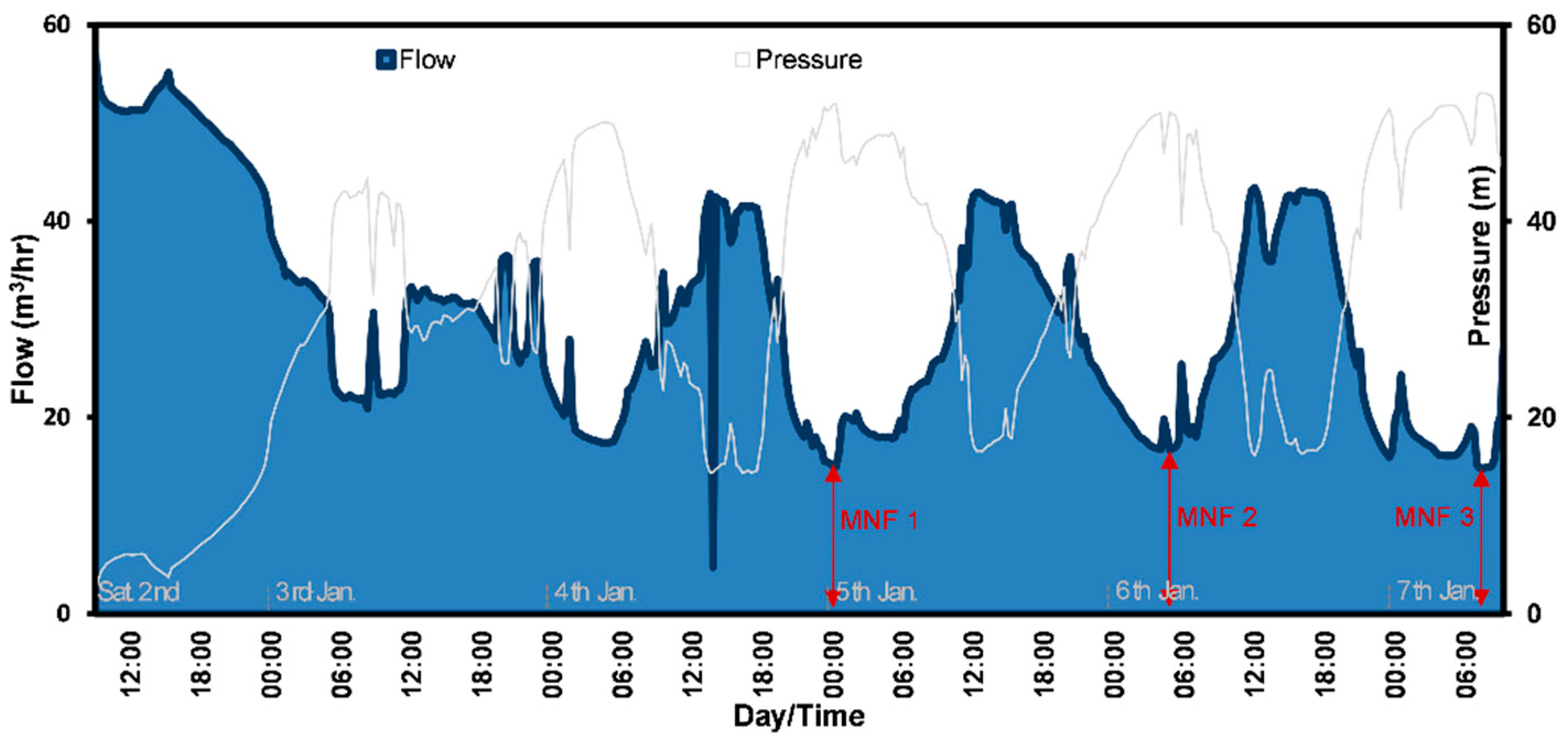
Figure 3 shows the pressure and flow measurements in the DMA during the period of the experiment. Figure 3a shows the logged pressures in three points: the inlet point, a med-elevation point and a high-elevation point, showing the range of the pressure in the DMA. Pressure of the DMA ranges from 6.0 to 60.0 meters with a mean of 32.4 m and 14 m standard deviation.
Figure 3b shows the measured pressures in two other points that lie between the same range in Figure 3a, but with a pressure drop at med 2 point on Monday, 4 January 2016 from 9:00 a.m. until 18:00 p.m. This pressure drops coincided with a flow drop from 43 to 5 m3/h on the same day (Figure 3c) due to a probable change in a valve situation, but shortly recovered in the records of the next 15 min. The flow and pressure drops are highlighted in the right-side of Figure 3. The experiment however succeeded to reach the saturation level on the following three days which are used for the MNF analysis: Tuesday, Wednesday and Thursday, which were 5, 6 and 7 January 2016, respectively. The saturation status was reached on the third day, after 63 h (2.63 days) of continuous supply. By that time the water entering the DMA satisfied the demand and all ground and elevated tanks were full, and the records started to closely repeat themselves for three consecutive days, enabling analysis of the leakage rate in the DMA. Figure 3c shows the typical demand-pressure relationship in the DMA where the pressure (mean) drops down when there is high demand and rises when there is less demand, during night or morning time.
Figure 4 shows the leakage-pressure modelling based on the pressure measurements. Firstly, the legitimate night consumption () was deduced from the MNF rate, and then the leakage rate of this specific time was calculated. As the MNF time lasts for 1.5 h, was divided by the same value, to give the hourly which is used to calculate the leakage rate at the MNF time (Equation (1)). Secondly, the hourly leakage volume during the day was modelled as shown in Figure 4 using the FAVAD concept, and thirdly the daily leakage volume was calculated based on the night day factor (Equations (5) and (6)). The leakage volume in the DMA was 882 m3 for the period of the experiment, which is 24.1% of the water supplied into the DMA. Table 1 shows that if the legitimate night time consumption is altered or divided by two hours (instead of 1.5 h), the leakage rate increases to 927 m3, which is 25.4% of the supplied water. This indicates the sensitivity of the to the calculations. In this analysis, the values used for were 2.51 m3/h for 753 people using 5 L flush toilets during a period of 1.5 h. The used value of the MNF to calculate the daily leakage was almost similar on 5 and 7 January (average of the two days), and the calculated night day factor is 14.2 h/day. However, if the average MNF of the last three days is used, the leakage becomes 25.1% of the supplied water, indicating less sensitivity in the calculations than Additionally, Figure 5 also shows that time of the MNF occurred at 12:15 a.m., 4:45 a.m. and 7:15 a.m. for the last three days of the experiment, respectively. Similar cases were also reported in the literature [17]. This means that MNF can also occur even when part of the customer base is active (e.g., for Fajr prayer at 5:00 a.m. in January) as long as customers do not pump water from the ground to the elevated tanks during the MNF time.
Generalising the leakage level of AL-Hashimia DMA for the entire network depends on how representative the DMA is for the network. This process is associated with uncertainties on similarities and differences of asset and operating conditions in the network. The higher the number of DMAs experimented, the more representative the estimated level of leakage for the whole network, but is probably fully representative only if the entire network is divided into DMAs and MNF is carried out for all the DMAs. However, to have an annual estimate of the leakage level, MNF should be carried out regularly throughout the year for all the DMAs, as leakage could vary with the time. This is not technically, operationally and economically possible in the current situation in the Zarqa network. For this reason, the leakage level of the DMA was assumed to represent the entire Zarqa network, and further investigation of this assumption was eventually carried out.
Based on the MNF analysis, the leakage level of the network was estimated at 16.1 million m3/year. Further analysis for the leakage components was carried out through the Bursts and Background Estimates (BABE) using the breaks and failures records for each pipe diameter in the network. The response time to repair the reported or detected leaks was computed in the DC Maintenance Management System (DCMMS) with an annual average of 2 days in 2014. The detected leaks through leakage detection surveys were estimated for each pipe diameter with estimated awareness and repair times. Accordingly, the leakage from reported and unreported failures was estimated at 2.4 million m3/year. The background leakage was estimated at 1.8 million m3/year. The differences between the estimated leakage volume by the MNF analysis and the sum of these two volumes is considered as hidden losses, which are 11.8 million m3/year. It is not known how much of the hidden losses are the recoverable and unavoidable quantities. Obviously, the component analysis of leakage (BABE) analyses a small part of the leakage in this case. Although the Infrastructure Condition Factor was assumed at high level in the model (ICF = 2.5), the component analyses of the leakage model analysed only 26.3% of the leakage in Zarqa, and the remaining 73.6% is not analysed and thus considered as hidden losses. This is probably due to the empirical assumptions of flow and characteristics of bursts and unavoidable leakage in the BABE model that are not totally applicable for all cases. Altering the ICF to 5, the hidden losses remained at more than 60% of the leakage. This result emphasises the need for an adaptation study for the BABE model in the intermittent supply context.
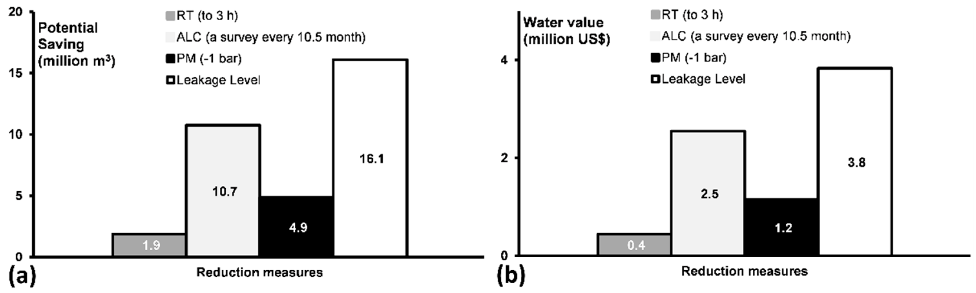
Based on the component analysis of leakage, the savings of the leakage reduction measures were analysed using the economic model: Component Analysis: a Tool for Economic Water Loss Control. Different scenarios for leakage reductions are possible in Zarqa. Figure 6 shows the potential water and monetary saving through different measures. Reducing the average response time of repairing the reported and detected leaks from 2 days to 3 h is a target of Zarqa utility. This would save 1.9 million m3/year with a monetary value of US$ 0.4 million, using the variable production cost in Zarqa. Adopting an Active Leakage Control (ALC) policy through regular leak detection surveys that complete the network every 10.5 months could save 10.7 million m3/year (US$ 2.5 million). Reducing the average pressure of the entire network from 33 m to 23 m, e.g., through separating the elevated parts of the network, would save 4.9 million m3/year (US$ 1.2 million). Nevertheless, the economic model analyses each of these measures independently while it is likely that these measures are dependent on each other, e.g., pressure reduction limits the failure frequencies and lowers the potential of ALC as leaks will be harder to detect. For this reason, aggregating the savings of the three measures is likely to overestimate the potential of the leakage reductions, e.g., the savings will be higher than the volume and value of the leakage. For this reason, it is worthwhile for future economic modelling of leakage to take into account the dependency of the different measures on each other.
To have an insight of the critical factors in the aforementioned economic model, the sensitivity of two factors were analysed. The rate of rise of unreported leakage (RR) was manipulated in the model for low, moderate and high values [58] and then the resulting savings were reported. This step was conducted for two levels of infrastructure condition factor, ICF = 1.5 and ICF = 2.5 as these two levels are suggested in the model. Figure 7a shows the impact of altering the RR on the water saving (left axis) and the monetary value (right axis) when adopting ALC through leakage detection surveys. At a low level of RR (e.g., 1 m3/km mains/day/year), 66% of the network has to be surveyed every year. The potential saving will then be 11.2 million m3/year (US$ 2.7 million) with a survey annual cost at US$ 0.15 million based on a survey cost of US$ 100/km. At a high level of RR (e.g., 5 m3/km mains/day/year), 147% of the network has to be surveyed every year. The potential savings will then be 10.4 million m3/year (US$ 2.5 million) with a survey annual cost at US$ 0.33 million. For a moderate rate (RR = 3 m3/km mains/day/year), 114% of the network has to be surveyed every year with a saving of 10.7 million m3/year (US$ 2.5 million). This analysis suggests the high sensitivity of RR in modelling the economic frequency of leakage detection surveys, which complicates the task in intermittent supplies where RR is difficult to estimate accurately. For this reason, the moderate level of RR was used in Zarqa and Figure 7a shows the model results for different RR values. Figure 7b shows the same parameters of Figure 7a but for ICF at 1.5, which is not very sensitive in the output of the economic model, and the figures are close to those in Figure 7a. Noticeably, more work is required to improve the reliability of the economic analysis of the leakage through fixing the rate of rise of the leakage and the component analysis of the leakage in intermittent supplies.
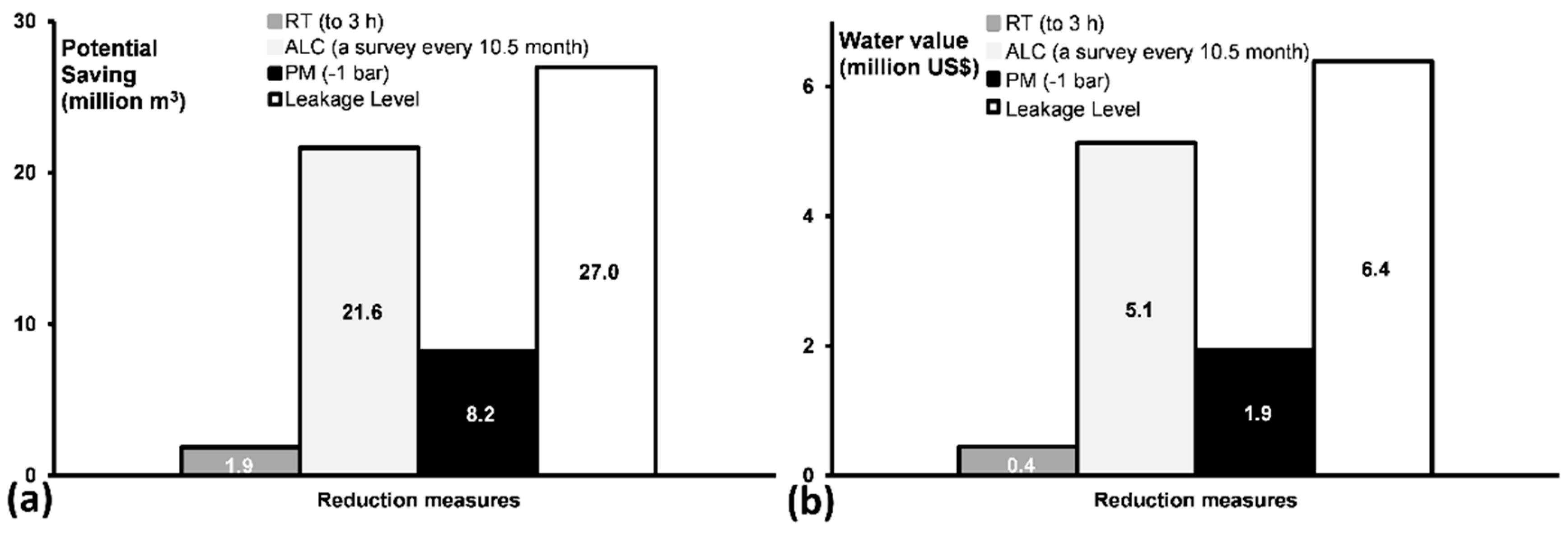
Finally, to suggest reliable outputs of the leakage reductions in the whole system, the overall volume of leakage was estimated through the top-down water balance and integrated with the MNF analysis [7]. Figure 8 shows the summary of the parameters discussed previously but with altering the volume of the leakage in the model to 26.9 million m3/year, which is the average result of estimating leakage volume through MNF analysis and top-down water balance. While MNF analysis is reasonably accurate at the DMA scale, upscaling its results for the entire system is uncertain and sensitive. Leakage estimation from one DMA is likely to be not sufficiently representative for the entire system. The overall annual volume of the leakage in a system should be verified through several methods, before it is used for leakage reduction modelling. In all cases, estimating the benefits of the ALC seems to be overestimated using Equation (8). Further investigation is required to confirm this issue, and also to clarify the dependency relationship between potential savings of ALC and pressure management.
4. Conclusions
4.1. Minimum Flow Analysis in Intermittent Supplies
- One-day minimum night flow analysis (MNF) cannot be used to estimate the leakage rate in intermittent supplies, because water keeps flowing during night time to fill customers’ tanks in the network. Therefore, the experimented zone (DMA) should be supplied continuously for several days until the zone is saturated, or the customer ground or elevated tanks in the network are completely full, and the readings start to closely repeat themselves.
- MNF could therefore occur at night or day time, even if part the customer base are active as long as the ground tanks are full and customers do not pump water from the ground to the elevated tanks. In Zarqa, the saturation of the DMA started after 63 h of continuous supply and MNF was occurring between 12:00 a.m. and 7:00 a.m. This challenge requires more careful estimation of the legitimate nighttime consumption that is found to be a sensitive parameter in leakage estimation and modelling.
- Generalising the leakage rate at the time of the MNF for all the time of the day causes overestimating of the daily leakage, because of the usually lower pressures during the day. For this reason, the night day factor in Zarqa is a reduction factor (<24 h/day), being 14 h/day.
- While MNF analysis is reasonably accurate at a DMA scale, upscaling its result for the entire system is uncertain and sensitive. One or several DMAs cannot satisfy the diversity of the operating conditions in the network in terms of pressure, flows, pipe length and the number of connections. Therefore, estimating the leakage of the whole system has to be verified through several methods before it is used for full-system leakage reduction modelling.
4.2. Leakage Reduction Modelling in Intermittent Supplies
- The leakage component analysis model (BABE) analyses only a small part of the leakage (26% in the Zarqa case) and the remaining part is considered as hidden losses where the recoverable and unavoidable portions are not known. Increasing the Infrastructure Condition Factor is not sufficiently influential in the studied case, and the model may require an adaptation study for the intermittent supply context.
- Analysing the potential water savings of different leakage reduction policies independently and separately is currently possible. However, this approach is likely overestimating the potential savings significantly, due to the inter-dependency of the different policies, leading the potential savings to be more than the volume and cost of the leakage. In all cases, estimating the benefits of the frequent leakage detection survey seems to be over-estimated, and further investigation is required to clarify and confirm this issue.
- The inter-dependency relationship between the pressure management and active leakage control should be investigated too. Pressure reduction limits the failure frequencies and lowers the potential of leakage detection as leaks become harder to detect. Therefore, future leakage reduction modelling would be more reasonable when considering the influence of a specific leakage reduction policy (e.g., pressure management) on the potential of other reduction policies (e.g., ALC).
Author Contributions
T.A.-W. and S.S. designed this research. T.A.-W. carried out this research with local partners. S.S. revised the analysis and the paper. F.A.-N. and M.H. conceived ideas in the field work and revised the paper. M.K. supervised and took part in the design, implementation, analysis and writing process.
Funding
This work was funded by NICHE 27 Project: MetaMeta Research, Water and Environment Centre in Sana'a University, Yemen, and The Dutch Organisation for Internationalisation in Education (NUFFIC).
Acknowledgments
The authors are thankful to Jordan Water Company—Zarqa for providing access to the data and for the technical support to carry out the field work. Zeyad Shawagfeh, Ryadh Alshaieb, Mohammed Alkhalailah, Muneer Owies and the leakage crew of the company are acknowledged for their contribution.
Conflicts of Interest
The authors declare no conflict of interest.
References
- Gong, W.; Suresh, M.A.; Smith, L.; Ostfeld, A.; Stoleru, R.; Rasekh, A.; Banks, M.K. Mobile sensor networks for optimal leak and backflow detection and localization in municipal water networks. Environ. Model. Softw. 2016, 80, 306–321. [Google Scholar] [CrossRef] [Green Version]
- AL-Washali, T.; Sharma, S.; Kennedy, M. Methods of Assessment of Water Losses in Water Supply Systems: A Review. Water Resour. Manag. 2016, 30, 4985–5001. [Google Scholar] [CrossRef]
- Dighade, R.; Kadu, M.; Pande, A. Challenges in water loss management of water distribution systems in developing countries. Int. J. Innov. Res. Sci. Eng. Technol. 2014, 3, 13838–13846. [Google Scholar]
- Meseguer, J.; Mirats-Tur, J.M.; Cembrano, G.; Puig, V.; Quevedo, J.; Pérez, R.; Sanz, G.; Ibarra, D. A decision support system for on-line leakage localization. Environ. Model. Softw. 2014, 60, 331–345. [Google Scholar] [CrossRef] [Green Version]
- Farley, M.; Trow, S. Losses in Water Distribution Networks; IWA Publishing: London, UK, 2003. [Google Scholar]
- AWWA. M36 Water Audits and Loss Control Programs, 4th ed.; American Water Works Association: Denver, CO, USA, 2016. [Google Scholar]
- Thornton, J.; Sturm, R.; Kunkel, G. Water Loss Control; McGraw Hill Professional: New York, NY, USA, 2008; ISBN 978-0071499187. [Google Scholar]
- Fanner, P. Assessing Real Water Losses: A Practical Approach; International Water Association, Water 21: London, UK, 2004; ISSN 15619508. [Google Scholar]
- Morrison, J.; Tooms, S.; Rogers, D. District Metered Areas, Guidance Notes; International Water Association (IWA), Specialist Group on Efficient Operation and Management of Urban Water Distribution Systems: London, UK, 2007. [Google Scholar]
- Lambert, A.; Hirner, W. Losses from Water Supply Systems: A Standard Terminology and Recommended Performance Measures; IWA Publishing: London, UK, 2000. [Google Scholar]
- Puust, R.; Kapelan, Z.; Savic, D.; Koppel, T. A review of methods for leakage management in pipe networks. Urban Water J. 2010, 7, 25–45. [Google Scholar] [CrossRef]
- Liemberger, R.; Farley, M. Developing a nonrevenue water reduction strategy Part 1: Investigating and assessing water losses. In Proceedings of the IWA Specialized Conference: The 4th IWA World Water Congress Marrakech, Marrakech, Morocco, 19–24 September 2004. [Google Scholar]
- Farah, E.; Shahrour, I. Leakage Detection Using Smart Water System: Combination of Water Balance and Automated Minimum Night Flow. Water Resour. Manag. 2017, 31, 4821–4833. [Google Scholar] [CrossRef]
- Latchoomun, L.; King, R.A.; Busawon, K. A new approach to model development of water distribution networks with high leakage and burst rates. Procedia Eng. 2015, 119, 690–699. [Google Scholar] [CrossRef]
- Eugine, M. Predictive Leakage Estimation using the Cumulative Minimum Night Flow Approach. Am. J. Water Resour. 2017, 5, 1–4. [Google Scholar]
- Werner, M.; Maggs, I.; Petkovic, M. Accurate measurements of minimum night flows for water loss analysis. In Proceedings of the 5th Annual WIOA NSW Water Industry Engineers & Operators Conference, Water Loss Management Program NSW, Exhileracing Events Centre, Newcastle, UK, 29–31 March 2011; pp. 31–37. [Google Scholar]
- Alkasseh, J.M.; Adlan, M.N.; Abustan, I.; Aziz, H.A.; Hanif, A.B.M. Applying minimum night flow to estimate water loss using statistical modeling: A case study in Kinta Valley, Malaysia. Water Resour. Manag. 2013, 27, 1439–1455. [Google Scholar] [CrossRef]
- Fantozzi, M.; Lambert, A. Legitimate night use component of minimum night flows initiative. In Proceedings of the IWA Water Loss Conference, São Paulo, Brazil, 6–9 June 2010. [Google Scholar]
- Hamilton, S.; McKenzie, R. Water Management and Water Loss; IWA Publishing: London, UK, 2014. [Google Scholar]
- Lambert, A. What do we know about pressure-leakage relationships in distribution systems. In Proceedings of the IWA Conference in Systems Approach to Leakage Control and Water Distribution System Management, Brno, Czech Republic, 16–18 May 2001. [Google Scholar]
- Thornton, J.; Lambert, A. Progress in practical prediction of pressure: Leakage, pressure: Burst frequency and pressure: Consumption relationships. In Proceedings of the IWA Specialised Conference ‘Leakage 2005’, Halifax, NS, Canada, 12–14 September 2005; pp. 12–14. [Google Scholar]
- Van Zyl, J.; Lambert, A.; Collins, R. Realistic Modeling of Leakage and Intrusion Flows through Leak Openings in Pipes. J. Hydraul. Eng. 2017, 143, 04017030. [Google Scholar] [CrossRef]
- Alonso, J.M.; Alvarruiz, F.; Guerrero, D.; Hernández, V.; Ruiz, P.A.; Vidal, A.M.; Martínez, F.; Vercher, J.; Ulanicki, B. Parallel computing in water network analysis and leakage minimization. J. Water Resour. Plan. Manag. 2000, 126, 251–260. [Google Scholar] [CrossRef]
- Wu, Z.Y.; Sage, P.; Turtle, D. Pressure-dependent leak detection model and its application to a district water system. J. Water Resour. Plan. Manag. 2009, 136, 116–128. [Google Scholar] [CrossRef]
- Jowitt, P.W.; Xu, C. Optimal valve control in water-distribution networks. J. Water Resour. Plan. Manag. 1990, 116, 455–472. [Google Scholar] [CrossRef]
- Mazzolani, G.; Berardi, L.; Laucelli, D.; Martino, R.; Simone, A.; Giustolisi, O. A methodology to estimate leakages in water distribution networks based on inlet flow data analysis. Procedia Eng. 2016, 162, 411–418. [Google Scholar] [CrossRef]
- Mazzolani, G.; Berardi, L.; Laucelli, D.; Simone, A.; Martino, R.; Giustolisi, O. Estimating Leakages in Water Distribution Networks Based Only on Inlet Flow Data. J. Water Resour. Plan. Manag. 2017, 143, 04017014. [Google Scholar] [CrossRef]
- Lambert, A.; Lalonde, A. Using practical predictions of economic intervention frequency to calculate short-run economic leakage level, with or without pressure management. In Proceedings of the IWA Specialised Conference ‘Leakage 2005’, Halifax, NS, Canada, 12–14 September 2005; pp. 310–321. [Google Scholar]
- Lambert, A.; Fantozzi, M. Recent advances in calculating economic intervention frequency for active leakage control, and implications for calculation of economic leakage levels. Water Sci. Technol. Water Supply 2005, 5, 263–271. [Google Scholar] [CrossRef]
- Lambert, A.; Charalambous, B.; Fantozzi, M.; Kovac, J.; Rizzo, A.; St John, S.G. 14 years’ experience of using IWA best practice water balance and water loss performance indicators in Europe. In Proceedings of the IWA Specialized Conference: Water Loss 2014, Vienna, Austria, 31 March–2 April 2014. [Google Scholar]
- Lambert, A.; Brown, T.G.; Takizawa, M.; Weimer, D. A review of performance indicators for real losses from water supply systems. J. Water Supply Res. Technol. AQUA 1999, 48, 227–237. [Google Scholar] [CrossRef]
- Amoatey, P.; Minke, R.; Steinmetz, H. Leakage estimation in developing country water networks based on water balance, minimum night flow and component analysis methods. Water Pract. Technol. 2018, 13, 96–105. [Google Scholar] [CrossRef]
- AL-Washali, T.; Sharma, S.; Kennedy, M.; AL-Nozaily, F.; Haidera, M. Monitoring the Non-Revenue Water Performance in Intermittent Supplies. Water Resour. Manag 2019. in preparation. [Google Scholar]
- Di Nardo, A.; Di Natale, M.; Santonastaso, G.F.; Venticinque, S. An automated tool for smart water network partitioning. Water Resour. Manag. 2013, 27, 4493–4508. [Google Scholar] [CrossRef]
- Galdiero, E.; De Paola, F.; Fontana, N.; Giugni, M.; Savic, D. Decision support system for the optimal design of district metered areas. J. Hydroinform. 2015, 18, 49–61. [Google Scholar] [CrossRef] [Green Version]
- Kesavan, H.; Chandrashekar, M. Graph-theoretical models for pipe network analysis. J. Hydraul. Div. 1972, 98, 345–364. [Google Scholar]
- Deuerlein, J.W. Decomposition model of a general water supply network graph. J. Hydraul. Eng. 2008, 134, 822–832. [Google Scholar] [CrossRef]
- Di Nardo, A.; Di Natale, M.; Di Mauro, A. Water Supply Network District Metering: Theory and Case Study; Springer Science & Business Media: Berlin, Germany, 2013. [Google Scholar]
- Herrera, M.; Izquierdo, J.; Pérez-García, R.; Ayala-Cabrera, D. Water supply clusters by multi-agent based approach. In Water Distribution Systems Analysis 2010, Proceedings of 12th Annual Conference on Water Distribution Systems Analysis, Tucson, AZ, USA, 12–15 September 2010; pp. 861–869.
- Perelman, L.; Ostfeld, A. Topological clustering for water distribution systems analysis. Environ. Model. Softw. 2011, 26, 969–972. [Google Scholar] [CrossRef]
- Creaco, E.; Pezzinga, G. Multiobjective optimization of pipe replacements and control valve installations for leakage attenuation in water distribution networks. J. Water Resour. Plan. Manag. 2014, 141, 04014059. [Google Scholar] [CrossRef]
- De Paola, F.; Fontana, N.; Galdiero, E.; Giugni, M.; Savic, D.; Sorgenti degli Uberti, G. Automatic multi-objective sectorization of a water distribution network. Procedia Eng. 2014, 89, 1200–1207. [Google Scholar] [CrossRef]
- Fantozzi, M.; Lambert, A. Residential night consumption–assessment, choice of scaling units and calculation of variability. In Proceedings of the IWA Water Loss Conference, Manila, Philippines, 26–29 February 2012; pp. 26–29. [Google Scholar]
- May, J. Pressure Dependent Leakage; World Water and Environmental Engineering, Water Environment Federation: Washington, DC, USA, 1994. [Google Scholar]
- Lambert, A. Pressure management/leakage relationships: Theory, concepts and practical applications. In Proceedings of the IQPC Seminar, London, UK, April 1997. [Google Scholar]
- McKenzie, R.S. Water Demand Management Cookbook; Rand Water: Johannesburg, South Africa, 2003. [Google Scholar]
- Lambert, A.; Fantozzi, M.; Shepherd, M. FAVAD Pressure & Leakage:How Does Pressure Influence N1? In Proceedings of the IWA Water Efficient 2017 Conference, Bath, UK, 18–20 July 2017. [Google Scholar]
- Van Zyl, J.; Cassa, A. Modeling elastically deforming leaks in water distribution pipes. J. Hydraul. Eng. 2014, 140, 182–189. [Google Scholar] [CrossRef]
- Di Nardo, A.; Di Natale, M.; Gisonni, C.; Iervolino, M. A genetic algorithm for demand pattern and leakage estimation in a water distribution network. J. Water Supply Res. Technol. Aqua. 2015, 64, 35–46. [Google Scholar] [CrossRef]
- Lambert, A. Fast Track NDF Calculations Using the Correction Factor Method. Available online: http://www.leakssuite.com/night-day-factor-update/ (accessed on 9 December 2018).
- Kanakoudis, V.; Tsitsifli, S.; Papadopoulou, A. Integrating the carbon and water footprints’ costs in the water framework directive 2000/60/EC full water cost recovery concept: Basic principles towards their reliable calculation and socially just allocation. Water 2012, 4, 45–62. [Google Scholar] [CrossRef]
- Ashton, C.; Hope, V. Environmental valuation and the economic level of leakage. Urban Water 2001, 3, 261–270. [Google Scholar] [CrossRef]
- Pearson, D.; Trow, S. Calculating economic levels of leakage. In Proceedings of the IWA Water Loss 2005 Conference, Halifax, NS, Canada, 12–14 September 2005. [Google Scholar]
- Lambert, A. Accounting for losses: The bursts and background concept. Water Environ. J. 1994, 8, 205–214. [Google Scholar] [CrossRef]
- Sturm, R.; Gasner, K.; Wilson, T.; Preston, S.; Dickinson, M.A. Real Loss Component Analysis: A Tool for Economic Water Loss Control; Water Research Foundation: Denver, CO, USA, 2014. [Google Scholar]
- Aboelnga, H.; Saidan, M.; Al-Weshah, R.; Sturm, M.; Ribbe, L.; Frechen, F.-B. Component analysis for optimal leakage management in Madaba, Jordan. J. Water Supply Res. Technol.-Aqua 2018, 67, 384–396. [Google Scholar] [CrossRef]
- Fanner, P.; Thornton, J. The importance of real loss component analysis for determining the correct intervention strategy. In Proceedings of the IWA Water Loss 2005 Conference, Halifax, NS, Canada, 12–14 September 2005. [Google Scholar]
- Fanner, P.; Lambert, A. Calculating SRELL with pressure management, active leakage control and leak run-time options, with confidence limits. In Proceedings of the 5th IWA Water Loss Reduction Specialist Conference, Cape Town, South Africa, 26–30 April 2009; pp. 373–380. [Google Scholar]
Figure 1.
Map of Zarqa water network showing AL-Hashimiah DMA and positions of the data loggers (inset).
Figure 1.
Map of Zarqa water network showing AL-Hashimiah DMA and positions of the data loggers (inset).

Figure 2.
Data loggers for pressure measurements.

Figure 3.
Flow and pressure measurements in the DMA: (a) range of pressure in the DMA; (b) pressure measurement in further two points in the DMA with pressure collapse in one point; (c) flow and average pressure relationship in the DMA.
Figure 3.
Flow and pressure measurements in the DMA: (a) range of pressure in the DMA; (b) pressure measurement in further two points in the DMA with pressure collapse in one point; (c) flow and average pressure relationship in the DMA.

Figure 4.
Leakage modelling in AL-Hashimia DMA, Zarqa.

Figure 5.
Time of MNF occurrence in the DMA.

Figure 6.
Potential water saving of different leakage reduction measures. (a) volume of water saving (b) value of water saving.
Figure 6.
Potential water saving of different leakage reduction measures. (a) volume of water saving (b) value of water saving.

Figure 7.
Sensitivity of rate of rise of unreported leakage: (a) infrastructure condition factor = 2.5; (b) infrastructure condition factor = 1.5.
Figure 7.
Sensitivity of rate of rise of unreported leakage: (a) infrastructure condition factor = 2.5; (b) infrastructure condition factor = 1.5.

Figure 8.
Potential water saving of different leakage reduction measures through top-down water balance & MNF. (a) volume of water saving (b) value of water saving.
Figure 8.
Potential water saving of different leakage reduction measures through top-down water balance & MNF. (a) volume of water saving (b) value of water saving.


Table 1.
Sensitivities of the parameters of leakage volume estimation.
| Date | MNF | MNF Time | LNC | LNC Duration | NNL | NDF | Daily Leakage | Leakage Volume | Leakage Level |
|---|---|---|---|---|---|---|---|---|---|
| m3/h | a.m. | m3/h | h | m3/h | h/day | m3/day | m3 | % SIV | |
| 5 January | 15.0 | 12:15 | 1.88 | 2.0 | 13.1 | 14.2 | 185.8 | 932.7 | 25.5% |
| 2.51 | 1.5 | 12.5 | 14.2 | 176.9 | 888.1 | 24.3% | |||
| 6 January. | 16.4 | 4:45 | 1.88 | 2.0 | 14.5 | 14.2 | 205.0 | 1029.4 | 28.2% |
| 2.51 | 1.5 | 13.9 | 14.2 | 196.2 | 984.8 | 26.9% | |||
| 7 January. | 14.8 | 7:15 | 1.88 | 2.0 | 13.0 | 14.2 | 183.5 | 921.3 | 25.2% |
| 2.51 | 1.5 | 12.3 | 14.2 | 174.6 | 876.7 | 24.0% | |||
| Average | 15.4 | - | 1.88 | 2.0 | 13.5 | 14.2 | 191.4 | 961.2 | 26.3% |
| 2.51 | 1.5 | 12.9 | 14.2 | 182.6 | 916.6 | 25.1% | |||
| Average 5 & 7 January | 14.9 | - | 1.88 | 2.0 | 13.0 | 14.2 | 184.6 | 927.0 | 25.4% |
| 2.51 | 1.5 | 12.4 | 14.2 | 175.8 | 882.4 | 24.1% |
© 2018 by the authors. Licensee MDPI, Basel, Switzerland. This article is an open access article distributed under the terms and conditions of the Creative Commons Attribution (CC BY) license (http://creativecommons.org/licenses/by/4.0/).
Share and Cite
MDPI and ACS Style
AL-Washali, T.; Sharma, S.; AL-Nozaily, F.; Haidera, M.; Kennedy, M. Modelling the Leakage Rate and Reduction Using Minimum Night Flow Analysis in an Intermittent Supply System. Water 2019, 11, 48. https://doi.org/10.3390/w11010048
AMA Style
AL-Washali T, Sharma S, AL-Nozaily F, Haidera M, Kennedy M. Modelling the Leakage Rate and Reduction Using Minimum Night Flow Analysis in an Intermittent Supply System. Water. 2019; 11(1):48. https://doi.org/10.3390/w11010048
Chicago/Turabian StyleAL-Washali, Taha, Saroj Sharma, Fadhl AL-Nozaily, Mansour Haidera, and Maria Kennedy. 2019. "Modelling the Leakage Rate and Reduction Using Minimum Night Flow Analysis in an Intermittent Supply System" Water 11, no. 1: 48. https://doi.org/10.3390/w11010048
Note that from the first issue of 2016, this journal uses article numbers instead of page numbers. See further details here.