The Influence of Flow Projection Errors on Flood Hazard Estimates in Future Climate Conditions


1
Institute of Geophysics Polish Academy of Sciences, Ks. Janusza 64, 01-542 Warsaw, Poland
2
Faculty of Civil and Environmental Engineering, University of Life Sciences (WULS-SGGW), Nowoursynowska 166, 02-787 Warsaw, Poland
*
Author to whom correspondence should be addressed.
Water 2019, 11(1), 49; https://doi.org/10.3390/w11010049
Submission received: 16 November 2018
/
Revised: 13 December 2018
/
Accepted: 18 December 2018
/
Published: 29 December 2018
(This article belongs to the Special Issue Extreme Floods and Droughts under Future Climate Scenarios)
Abstract
:The continuous simulation approach to assessing the impact of climate change on future flood hazards consists of a chain of consecutive actions, starting from the choice of the global climate model (GCM) driven by an assumed CO2 emission scenario, through the downscaling of climatic forcing to a catchment scale, an estimation of flow using a hydrological model, and subsequent derivation of flood hazard maps with the help of a flow routing model. The procedure has been applied to the Biala Tarnowska catchment, Southern Poland. Future climate projections of rainfall and temperature are used as inputs to the precipitation-runoff model simulating flow in part of the catchment upstream of a modeled river reach. An application of a lumped-parameter emulator instead of a distributed flow routing model, MIKE11, substantially lowers the required computation times. A comparison of maximum inundation maps derived using both the flow routing model, MIKE11, and its lump-parameter emulator shows very small differences, which supports the feasibility of the approach. The relationship derived between maximum annual inundation areas and the upstream flow of the study can be used to assess the floodplain extent response to future climate changes. The analysis shows the large influence of the one-grid-storm error in climate projections on the return period of annual maximum inundation areas and their uncertainty bounds.
1. Introduction
Following the EU Floods Directive (2007) [1], flood risk maps should take into account climate changes and should be updated in cycle, every six years. A standard approach to deriving flood risk maps, applied in Poland, consists of running the 1D MIKE11 model for design flood waves of different return periods (e.g., 500, 100, 10 years). Water management and adaptation to floods in Poland for a 100-year flood have been planned. Design flood wave and model simulations have been applied to estimate 100-year inundation outlines [2]. In flood risk assessment, a design flood is customarily applied when flow data are available. When annual flow series are short, event-based simulation approaches can be applied [3]. This type of approach uses a rainfall generator as an input to a rainfall–runoff model. Annual maximum flow events are subsequently selected from the obtained flow series and used as inputs to a 1-D hydraulic model to derive maximum inundation maps. Due to the relatively large computation time requirements of a distributed flow routing model, a continuous simulation approach is rarely applied to flood risk assessments [4].
In order to provide flood risk maps for the future, there is a need to include future climate projections in the design of a flood wave [5,6]. The design flood is usually estimated from the probability distribution of annual maximum flows, which may be influenced by water engineering structures or urbanization [7]. Human interference at the river side changes the water balance of the river and the character of flood events. The above-mentioned factors make flood frequency analysis (FFA) based on annual peak flows under the assumption of stationarity not very robust when future climatic and human-induced changes are expected. In addition, the standard approach assumes that, for example, a 1-in-100 year flow quantile will be transformed into a 1-in-100 year inundation extent. That assumption imposes the existence of a linear transformation between the flow and an inundation area downstream, which is not usually met in practice.
The other approach, followed here, consists of a continuous simulation of a climate projection–runoff–flow routing system for an ensemble of climate projections for the entire length of available records and direct derivation of the 1-in-100 year flood inundation maps. The possible scenarios of the flood protection schemes and changes in land use (e.g., urbanization) may be taken into account [8]. This approach avoids both drawbacks of the standard method, but may require a high amount of computing time, which will increase when the uncertainty of simulations is to be included in the derived risk maps.
The important point related to flood wave design, which includes three flood wave parameters (wave height, height, length and base level), is the uncertainty. This uncertainty might undermine the usefulness of the flood risk assessment [9,10,11,12]. In addition, an analysis of the influence of different adaptation scenarios requires an application of a distributed flow routing model that takes most of the computing time in the simulation approach.
In order to facilitate the computations, we propose an emulator of the 1D MIKE11 model. An emulator is a simple model approximating particular actions of the original model and is used instead of that model for computationally intensive applications. Two main types of emulators can be distinguished: structure-based emulators, where the mathematical structure of the emulator is derived from the simplifications of the original model, and data-based emulators, where the emulator structure is identified and its parameters estimated from a dataset generated from planned experiments performed on the complex simulation model [13].
The distributed 1D model of a riverside, treated as a complex model, can be successfully solved by data-based dynamic emulation modeling within the following steps [12]: (i) parameter estimation by calibration and validation of the emulator, (ii) analysis of the uncertainty of the output, and (iii) assimilation of the data to be analyzed within the emulator with defined parameters. The results of the emulator can be treated as an input to the flood risk assessment, which constitutes the basis for scenario analysis and a contribution to the decision-making process.
Decision-making with respect to adaptation or mitigation is usually based on flood risk assessments, which can be burdened by a quite high uncertainty [14]. This uncertainty can be divided into two groups: reducible and non-reducible. The reducible uncertainty is dependent on the amount of available information applied to the model, whereas the non-reducible uncertainty comes from the randomness of nature.
In Poland, even though the EU Floods Directive (2007) commits all EU countries to follow “the flood risk adaptation cycle,” the new Polish Water Act gives a high degree of freedom to meet the EU requirements and interpret the Act in different ways [15]. Since 1 January 2018, the responsibility for decision-making has been in the hands of local government. Local government bases its decision on existing master plans, and the regional flood prevention assessments usually do not contain an uncertainty analysis. At the county scale, the risk assessment seems to be no longer necessary, and the same refers to scenarios for adaptation.
The propagation of uncertainty [16,17] in the routing model begins at the stage of climate projection. Both global and regional climate projections display systematic errors [18,19]. Projections of temperature and precipitation data used as an input to a hydrological model may be over- or underestimated due to the climate model characteristics and bias related to downscaling [20,21].
The aim of this study is an assessment of the sensitivity of projections of annual maximum inundation area to climate projections and modeling errors, including rainfall–runoff and flow routing models. The analysis framed by this article in the context of Floods Directive 2007 satisfies the flood hazard assessment, which is an inherent part of flood risk assessment, enriched by the projection of future climate and uncertainty analysis but without cost–benefit analysis.
The Biala Tarnowska catchment in Southern Poland was used as a case study. Future projections of precipitation and temperature obtained from the EURO-CORDEX project were applied as inputs to the HBV model simulating flow in the upper part of the catchment, at the Ciezkowice gauging station. The sensitivity of the derived future inundation areas at Tuchow meander on the Biala River to climate projection errors was assessed.
The following content is organized within sections that present the methodology, describe the case study area, describe the emulator, discuss the results and the uncertainty of the results of both MIKE11 and the emulator of MIKE11, and apply the developed procedure to climate projections. Final comments on the achievements of this work are given in the conclusions.
2. Materials and Methods
2.1. Approach
The approach can be summarized in the following steps:
- calibration and validation of a distributed model (MIKE11) for the chosen river reach;
- development of an emulator for the selected cross sections of the model in the form of the input–output transformation;
- verification of the emulator using independent observation sets;
- comparison of the deterministic inundation extent maps obtained using both approaches;
- estimation of prediction error bands (uncertainty analysis of a flow routing model);
- derivation of dependence of annual maximum inundation area on the upstream flow;
- dependence of distribution of future annual maximum inundation areas on climate model instabilities.
The first step required the development of a distributed model for a selected river reach, using the available DTM data and measured cross sections. The choice of MIKE11 was dictated by the need to compare the results of modeling to the existing, MIKE11-based flood risk maps for the region of Biala Tarnowska.
In the second step, the emulator structure was developed based on the modeling goals and the characteristics of the processes involved [22]. The emulator calibration (Step 3) applied MIKE11 simulations as a source of information on unobserved water levels at cross sections along the river reach. Verification of the emulator (Step 4) was performed using the reference data from the time period not applied in the calibration stage. A comparison of the deterministic inundation extent maps provided an insight into the quality of the emulator spatial predictions. In the next step (5), the uncertainty of emulator predictions was assessed. The emulator was treated in this step as an additional source of errors, apart from the error related to the distributed flow routing model. We investigated the differences between MIKE11 predictions and the emulator predictions for the observations at Koszyce Wielkie. However, we cannot assess errors at unobserved cross sections, unless we have additional spatial data, even in the form of historical inundation maps. It would be possible to calculate the parametric errors by sampling MIKE11 roughness parameter space and derivation in the emulator for each sample. As there are already many studies on distributed model uncertainties [23], we focused on uncertainties related to the emulator itself. We considered observations of water levels at the Koszyce Wielkie gauging station to evaluate the emulator performance and its predictive uncertainty. The sixth step involved the derivation of a functional dependence (sensitivity curve) between maximum inundation area and the upstream flow based on the calibration data. The seventh step involved a comparison of the frequency distribution of the maximum annual inundation areas based on future climate projections with and without one-grid-storms caused by regional model instabilities.
2.2. Case Study—The Biala Tarnowska Catchment
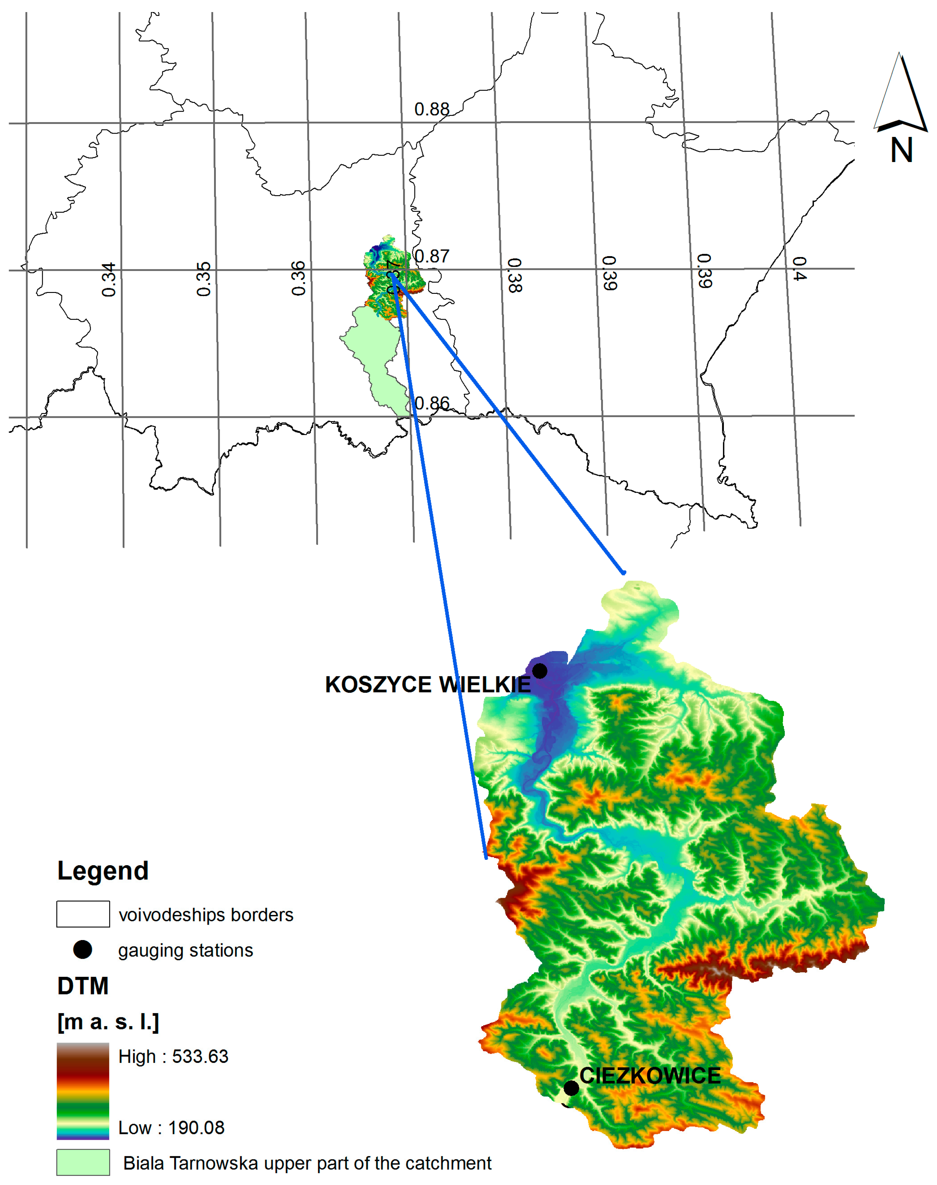
The Biala Tarnowska catchment, chosen as a case study, is a mountainous catchment in Southern Poland. The catchment is semi-natural, and one of the semi-natural Polish catchments, chosen following an extensive analysis of available hydro-meteorological and geomorphological data [24]. The catchment, with an area of 966.9 km2, has a forest-covered upper part and a lower part covered mainly by agricultural lands (Figure 1).
The upper part of the catchment, down to the Ciezkowice gauging station (527.5 km2) with 97% classified as forest cover, was modeled by the HBV rainfall–runoff model.
Thiessen polygons were applied to interpolate point precipitation data for the purpose of rainfall–runoff model calibration and verification. The lower part of the river between Ciezkowice and Koszyce Wielkie gauging stations was modeled using the 1-D MIKE11 flow routing model and the emulator, based on a stochastic transfer function.
Daily hydro-metrological observations of precipitation, temperature, and streamflow and estimated potential evapotranspiration were used as an input to the hydrological model HBV [25]. Observed historical hydrological and climate daily time series of precipitation, temperature, and streamflow for 40 years from November 1970 to October 2010 were obtained from the National Water Resources and Meteorological Office (IMGW) in Poland. Daily potential evapotranspiration was calculated using the temperature-based Hamon approach [26]. Daily streamflow data from the Ciezkowice and Koszyce Wielkie hydrological stations for a period of 40 years (1971–2010) were used in the calibration (1971–2000) and validation (2001–2010) stages.
In the case of Biala Tarnowska, observations at the upstream gauging station Ciezkowice and the downstream, Koszyce Wielkie, show that one recording observations daily (6 a.m.) might miss the fast changes of flow in short flood events. The delay between observations in upstream and downstream is 8 h. Because of this, an additional check-up of input daily data was done by a comparison of 10 min observation data and interpolated daily data. The correlation between them was 0.93, which may lead to the conclusion that 1 h output results will contain the peaks of flood events.
2.3. Routing Model for Biala Tarnowska River
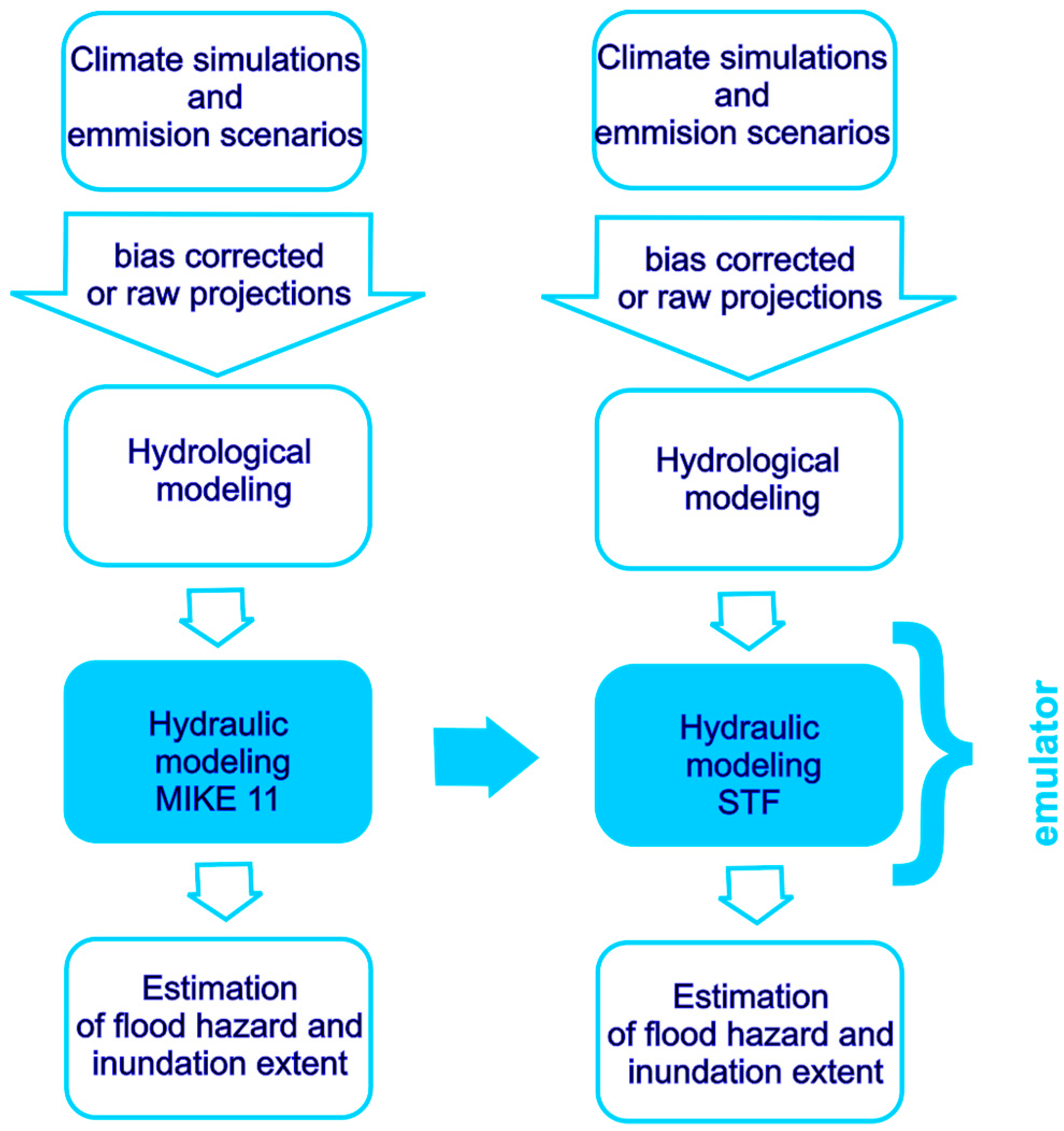
Two parallel approaches to modeling future inundation areas are presented schematically in Figure 2. The scheme shows the simulation chain of actions necessary to produce flood adaptation indices. At the left-hand side of Figure 2, the chain of actions starts from the input data (observed or simulated daily temperature and precipitation series), which are pre-processed for the whole time horizon of the simulations. They form the input to a hydrological model, which provides flow simulations subsequently routed using the MIKE11 model. The adaptation actions may consist of building the polder release at parts of the river reach to prevent downstream-located cities from flooding, building embankments, introducing levees, or other engineering constructions.
Distributed models, e.g., MIKE11 [27], SOBEK [28], and HEC-RAS [29], use the logic of a real-world system and follow the laws governing the routing of the river. Distributed flow routing is needed to test different adaptation measures and their influence on flood risk. However, modeling and comparison of the outcomes of flood adaptation measures require multiple simulations of the entire system, presented in the left panel of Figure 2.
The application of MIKE11 in this context requires a high amount of computing time. The approach proposed here consists of replacing the MIKE11 model by a transfer function-based emulator as shown in the right panel of Figure 2. The development of the emulator is based on the distributed model simulations, and its derivation is described in the following sub-sections.
The national climate change adaptation strategy for Poland, in the case of adaptation to floods, recommends the application of a top-down flow routing software—MIKE11 (DHI, Hørsholm, Denmark). For the sake of comparison of results, the same software has been chosen in this study.
The routing model of the Ciezkowice–Koszyce Wielkie reach of the Biala Tarnowska River includes 118 cross sections specified using the triple zone approach.
The triple zone approach defines the water depth border value and the resistance in each cross section. All cross sections were built using direct field measurements, and values were generated from the digital elevation model (DTM). The resolution of DTM is 1 m horizontally and 0.01 m vertically.
Due to the fact that, in the Biala Tarnowska reach, the water balance depends on ungauged tributaries in almost 50% of the total flow, the model was supplied with 19 point sources representing the tributaries and one lateral source. In our approach, we followed the discussion on lateral sources in the routing model presented in [30]. The authors show the impact of the saturated zone on matrix–conduit exchanges in a shallow phreatic aquifer and highlight the important role of the unsaturated zone on storage. In this work, flows of ungauged tributaries were estimated based on the HBV results for the whole Biala Tarnowska catchment and the participation of the tributary catchment areas in the Ciezkowice–Koszyce Wielkie part of the catchment. The flows do not take into account the delays caused by saturation but are simply weighted by the size of ungauged tributary sub-catchments.
The flow routing model has been simulated with a 1 min time step interval, using the HBV simulated flow time series for the period 1996–2000 as an upstream boundary condition and the rating curve as the downstream boundary. The fmincon optimisation routine from MATLAB® was applied to optimize six MIKE11 roughness parameters. The Nash–Sutcliff index (NS) was used to describe the goodness of model fit for the observed flows and water levels at the Koszyce Wielkie gauging station. The values of the NS index in Koszyce Wielkie, using flows as a criterion for the calibration and validation periods, were 0.80 and 0.77, respectively, whilst the NS indices for water levels were 0.60 and 0.54, respectively.
2.4. Input—The Hydrological Model for the Ciezkowice Gauging Station
In this study, the HBV hydrological model has been applied to the upper catchment of Biala Tarnowska (down to the Ciezkowice gauging station). The model applies daily temperature, evaporation and precipitation data as an input. The HBV [25] model parameters were optimized using the minimization code [31]. The parameters optimized by the are given in Table 1.
In addition, the HBV model was also used for the entire catchment closing at the Koszyce Wielkie gauging station to estimate the ungauged tributaries to the Biala reach between Ciezkowice and Koszyce Wielkie. The optimal model parameters for the whole catchment were obtained from [32] and are presented in Table 1.
2.5. The Structure of the MIKE11 Emulator
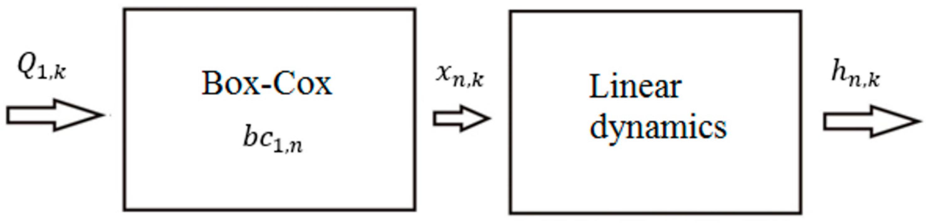
The emulator consists of a Box–Cox transform and a stochastic transfer function (STF) model [33]. The choice of the Box–Cox-STF-based model was dictated by its transparent structure combining nonlinear input transformation of the input variable (Box–Cox) with linear model dynamics (STF), forming the so-called Hammerstine-type model [34].
The emulator parameters are derived using the distributed model simulations, available at each model cross section and discrete in time. For the purpose of the derivation of flood inundation maps for future climate projections, the model input should have the form of flows, and model output should be in the form of water levels. Assuming that the emulator’s single module is built between the 1st and nth cross section, with the flow at an upstream end of the reach acting as an input variable, and the water levels at a cross section acting as an output variable, the system’s basic module has the structure as shown in Figure 3.
The emulator equation for the nth cross section has the form of a single-input single-output (SISO) model with the Box–Cox transformation of an input:
where denotes water levels at an MIKE11 cross section, denotes transformed by the Box–Cox model flow at the Ciezkowice cross section, and is the error. Parameters , , , , and are specific for each cross section.
The optimization of parameters of a Box–Cox transform was performed jointly with the STF model parameters, using the criterion to take into account the model output bias. From this point of view, the procedure was similar to the derivation of a nonlinear gain on the input in the flow forecasting model [34]. Its output can be expressed either in the form of flow or water levels at required spatial locations (e.g., the Koszyce Wielkie reach of the river).
It should be noted that any other suitable simplified flow routing model can be used as an emulator. The emulator with the STF describing process dynamics has the advantage of providing well-defined model parameters with a known covariance structure as part of its output. The nonlinear Box–Cox static transformation of flow is used to describe a nonlinear flow–water-level relationship and to improve the estimation of STF model parameters.
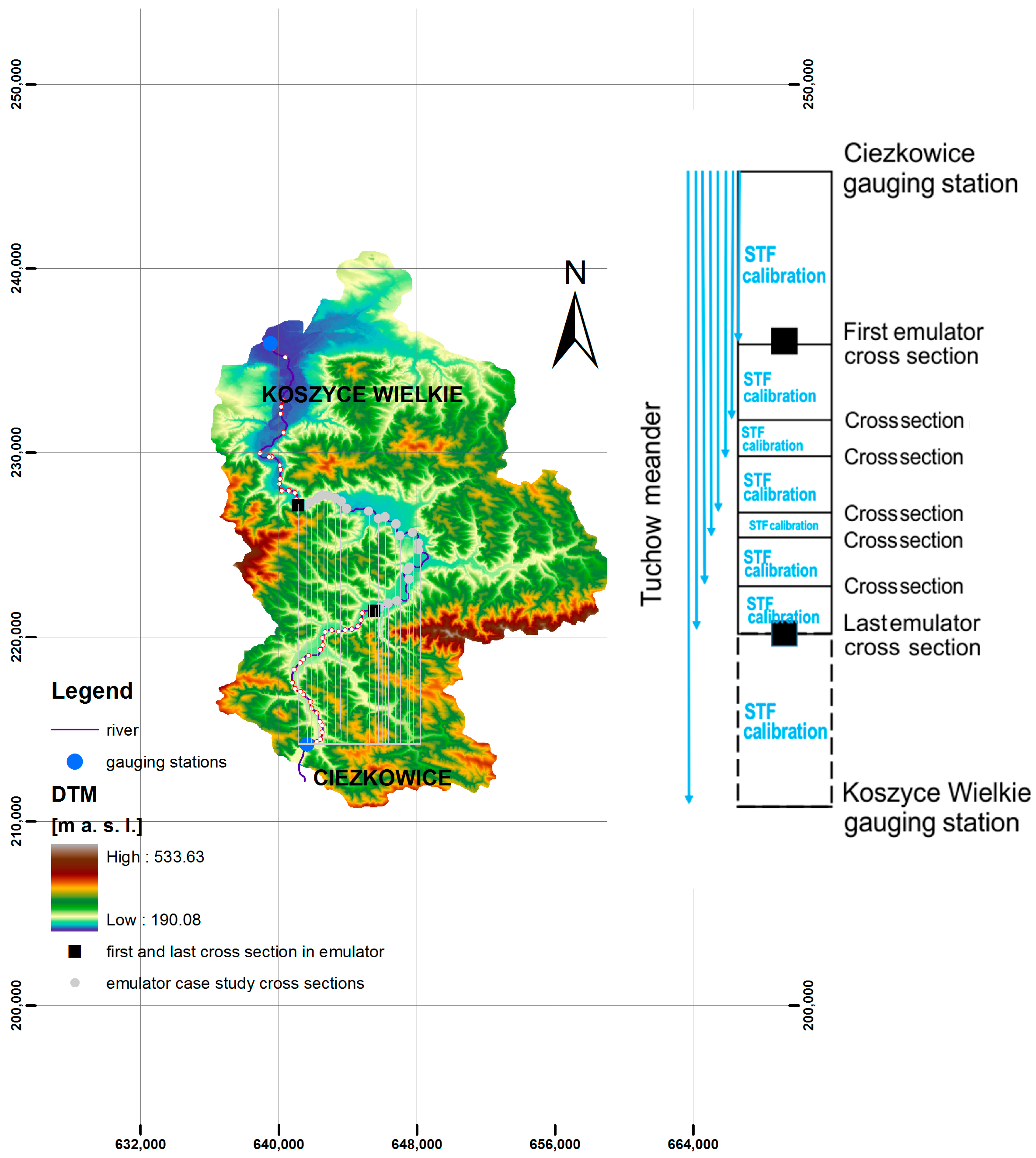
The emulator of a distributed flow routing model applied here has the form of parallel connected STF-type modules. The number of modules will depend on the number of cross sections required to build the inundation map, as shown in Figure 4. In the case study, 118 cross sections of the Biala River were used as components of the emulator. The part of the Ciezkowice–Koszyce reach includes the Tuchow meander, 16 km long, which will be used later as an illustration. It is shown by black squares in Figure 4 and consists of 38 cross sections. The emulator was optimized with the fminsearch function (part of the MATLAB function library), which applies the Nelder–Mead simplex method [35]. Both the NS index and were applied as objective functions evaluated at the vertices of a simplex. The adaptive nature of the process requires continuous revision of simplexes to find the best fit to the response surface. Each module is calibrated using the outputs (here the water levels at each cross section) obtained from the fully distributed model. The form of a module depends on the variable chosen to describe the system dynamics [22].
To take into account flood wave durations less than 24 h, hourly time steps were used for the estimation of emulator parameters. In the calibration stage, the best model fit in varied between 0.97 and 0.98, which shows a very good emulator performance. Besides the goodness of fit, the other parameters characterize the emulator. The pure advection delay between the first and the last Tuchow meander cross section is approximately 2 h, depending on the wave speed. However, the total time of wave propagation in the emulator from the beginning of the model to the last cross section of the meander was estimated at between 5 and 9 h [36]. The emulator well reproduces MIKE11 simulations, which is not surprising, as the input–output relationship between the distributed model variables is well defined. The accuracy of the validation expressed by the coefficient of determination is of a similar order as in the calibration stage (about 0.97). The total accuracy of the emulator predictions depends also on the MIKE11 accuracy, which can be tested at only one available gauging station: Koszyce Wielkie.
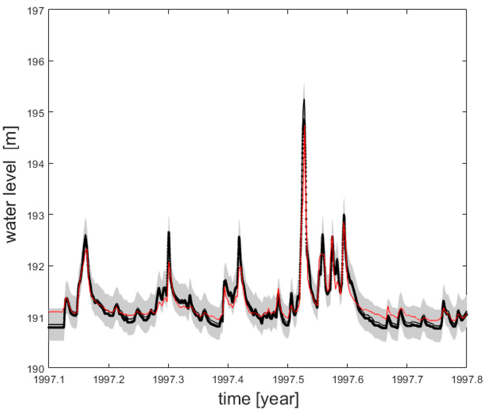
The results of the validation of water level predictions at the Koszyce Wielkie gauging station are presented in Figure 5. The emulator predictions are shown by a continuous black line together with 0.95 confidence bands depicted by the shaded area. The MIKE11 predictions are shown by the black dotted line, and the observed water levels are shown by the red line.
The SISO model could be introduced for Biala Tarnowska despite the tributaries present in the catchment due to the fact that they are strongly correlated with the main river flow. In the case where tributaries are not strongly correlated, the MISO (multiple-input single-output) approach is required [34].
3. Results
3.1. Comparison of Deterministic Flood Inundation Maps
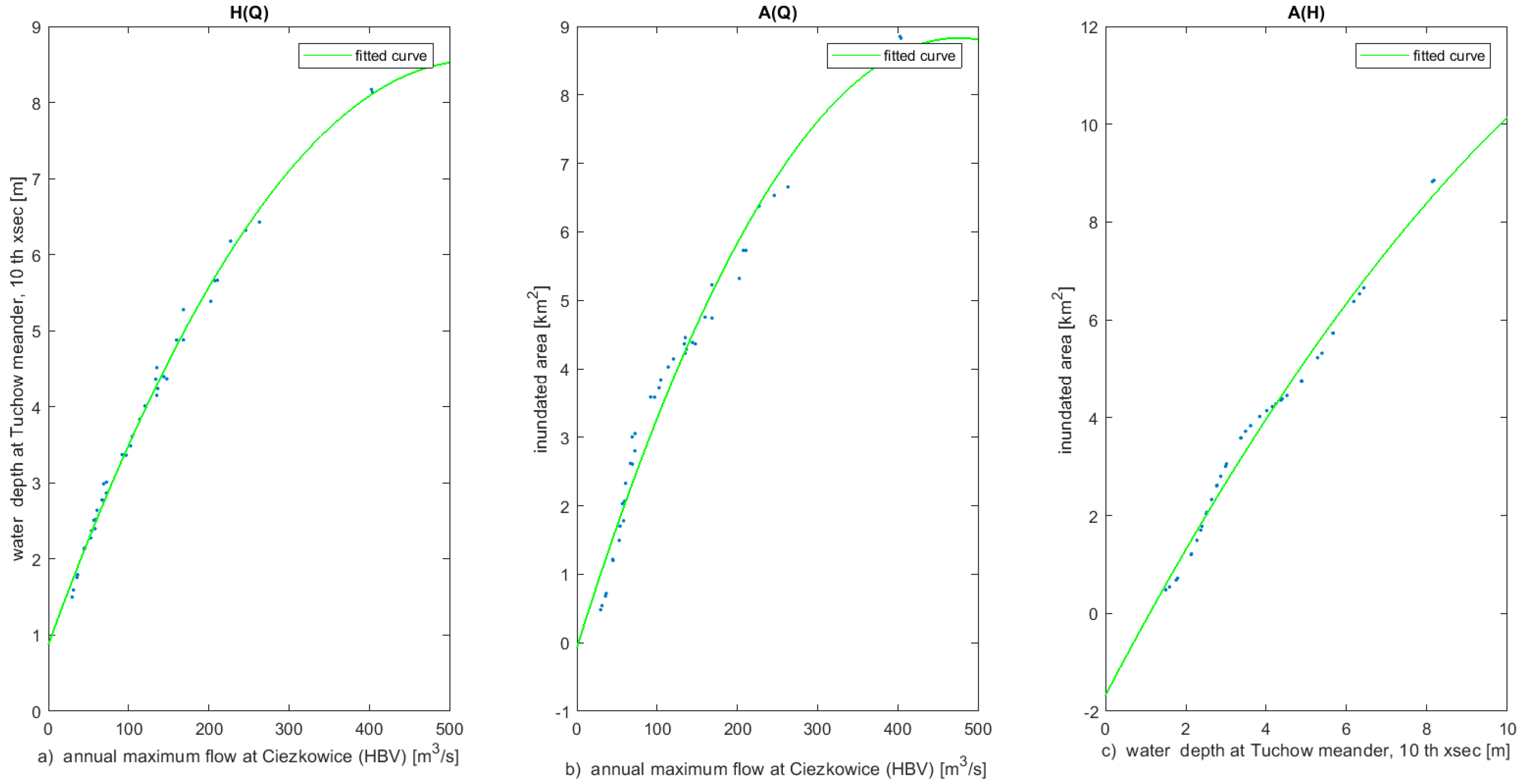
Flood inundation areas derived from the water level simulations of MIKE11 and the emulator are compared in the following subsection. The relationships between the annual maximum flow at Ciezkowice, forming the input to the emulator and corresponding water levels and inundation area at the Tuchow meander simulated by the emulator, are presented in Figure 6. The left-hand panel shows the relationship for the 10th meander cross section, the middle panel shows , and the right-hand panel shows the relationship between the water level at the 10th meander cross section and the meander annual maximum inundation area . The correlation coefficients of , and are 0.96, 0.98, and 0.99, respectively. In the plot (Figure 6, right hand panel), it can be seen that, for an increasing water depth value with a constant value of 1 m (dashed lines), the gradient of the inundated area changes. At a 5 m water depth, the embankments are exceeded, causing changes in the inundation area response.
The above illustration shows that relationships between the maximum inundation areas and inflow are nonlinear (middle panel of Figure 6). They can be used to derive local sensitivity indices describing how the inundation area responds to the variation in input flow at Ciezkowice for adaptation purposes. In particular, the relationship depends on the channel and floodplain geometry. In this case, the inundation area is more sensitive for smaller maximum flow values than for larger values.
The computation time of the emulator is much shorter than that of MIKE11. As illustrated in Table 2, the time of preparation of the inundation map using the emulator shows a difference of two orders of magnitude.
The vast amount of time might be consumed by mapping the water levels on the DTM. The time of mapping depends on the size of the area covered and its resolution, and it substantially influences the total computation time.
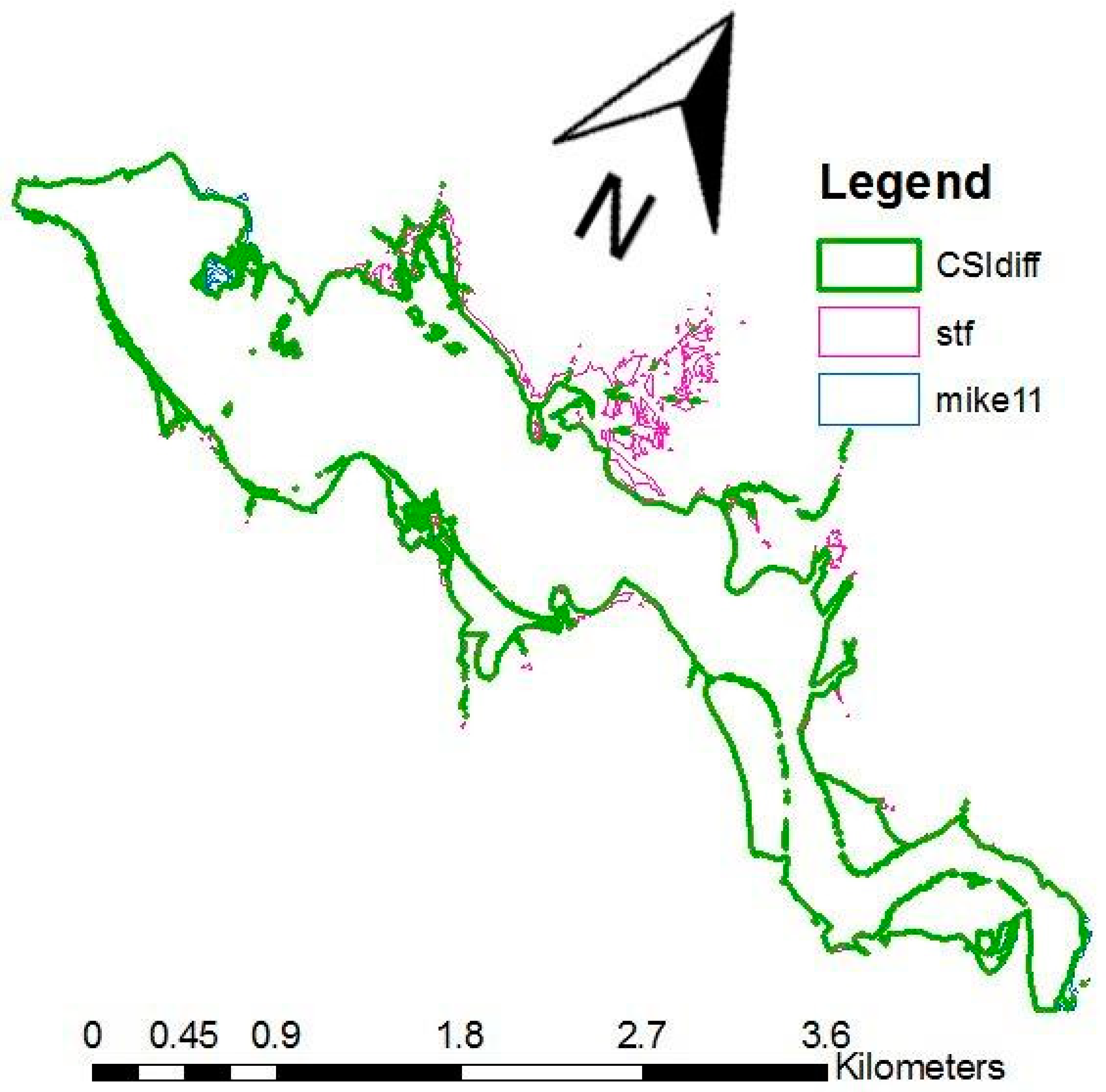
Figure 7 presents differences in the extent of maximum inundation area for the year 1997 for the lower part of the Tuchow meander. The emulator shows about 3.5% larger inundation area than MIKE11. The critical success index was used [37,38] to assess the differences quantitatively. The assumes that the times when an event is not expected and not observed have no consequence. The equation is as follows:
In this investigation, an is the inundation area simulated with the distributed MIKE11 model results, and the is that simulated with the results of the emulator of MIKE11 model. However, as spatial observations are missing, we do not know if MIKE11 under-predicts or over-predicts the real inundation extent.
The for the 1997 flood event equals 0.91. The application of the CSI eliminates grid cells that were differently classified by either of the approaches.
3.2. The Uncertainty of Emulator Predictions
The uncertainty of the emulator predictions depends on the uncertainty of the MIKE11 model predictions and on the emulator parametric uncertainties.
The uncertainty of the emulator of MIKE11 predictions can be assessed directly by comparison with the available observations. Unfortunately, no observations of either water levels or inundation extent are available along the modeled river reach, and only water levels at the gauging station in Koszyce Wielkie can be used for model validation and an estimation of the uncertainty of its predictions.
Following the standard STF model procedures, the model parameters, together with an estimate of their uncertainty and the prediction variance, were derived using the observations. When the MIKE11 model outputs were used instead of the measured values, the emulator prediction error was extended by the unknown error term, which also included the Box–Cox transform error.
Whilst the STF model parameter uncertainty is known for each MIKE11 cross section, the prediction error can be derived only for those cross sections where observations are available. Therefore, the STF model uncertainty describes the lower constraint (minimum value) of the uncertainty of the emulator predictions.
In order to estimate the influence of the Box–Cox transform and the STF model uncertainty on water levels generated by the emulator, we apply Monte Carlo simulations of the emulator parameters to generate an ensemble of possible model predictions. As each model provides the estimates of parameter uncertainty in the form of a covariance matrix, the simulations follow the information enclosed in those estimates. The procedure was applied to the Koszyce Wielkie gauging station. The model parameters and their uncertainty estimates are given in Table 3.
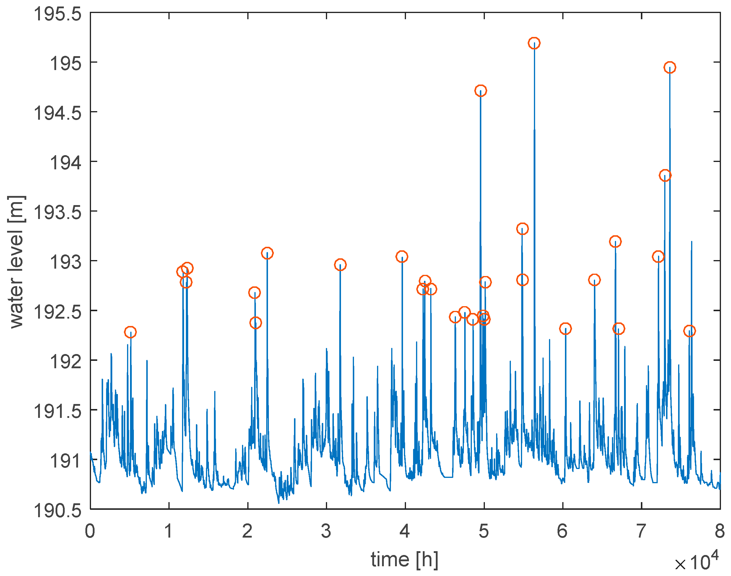
From the point of view of flood risk assessment, only the water level values that are above the bank-full are of interest. As the Koszyce Wielkie river reach has high embankments, the water level values that cause inundation upstream or downstream of Koszyce Wielkie are still in-bank at that cross section. In order to estimate their uncertainty related to the emulator parameters, the peak values above the 75th percentile (above 192 m) were selected from the generated ensemble of hourly water levels. The approach of [39] was followed in choosing the high-flow event series. The minimum distance between the events was set to 40 h, following the analysis of flow residence times to avoid the correlation between the events.
An example of event selection is presented in Figure 8. The correlation between the events was assessed using Bartlett’s test of independence for a significance level of 5%. As a result of that test, the independence assumption was not rejected.
The high flow events were used to derive the empirical water level-return-period curves following the approach described by [40].
The empirical return period of the i-th sorted highest peak water level was calculated from the ranked peak water level series according to the formula:
where denotes the number of years in a maximum water level series.
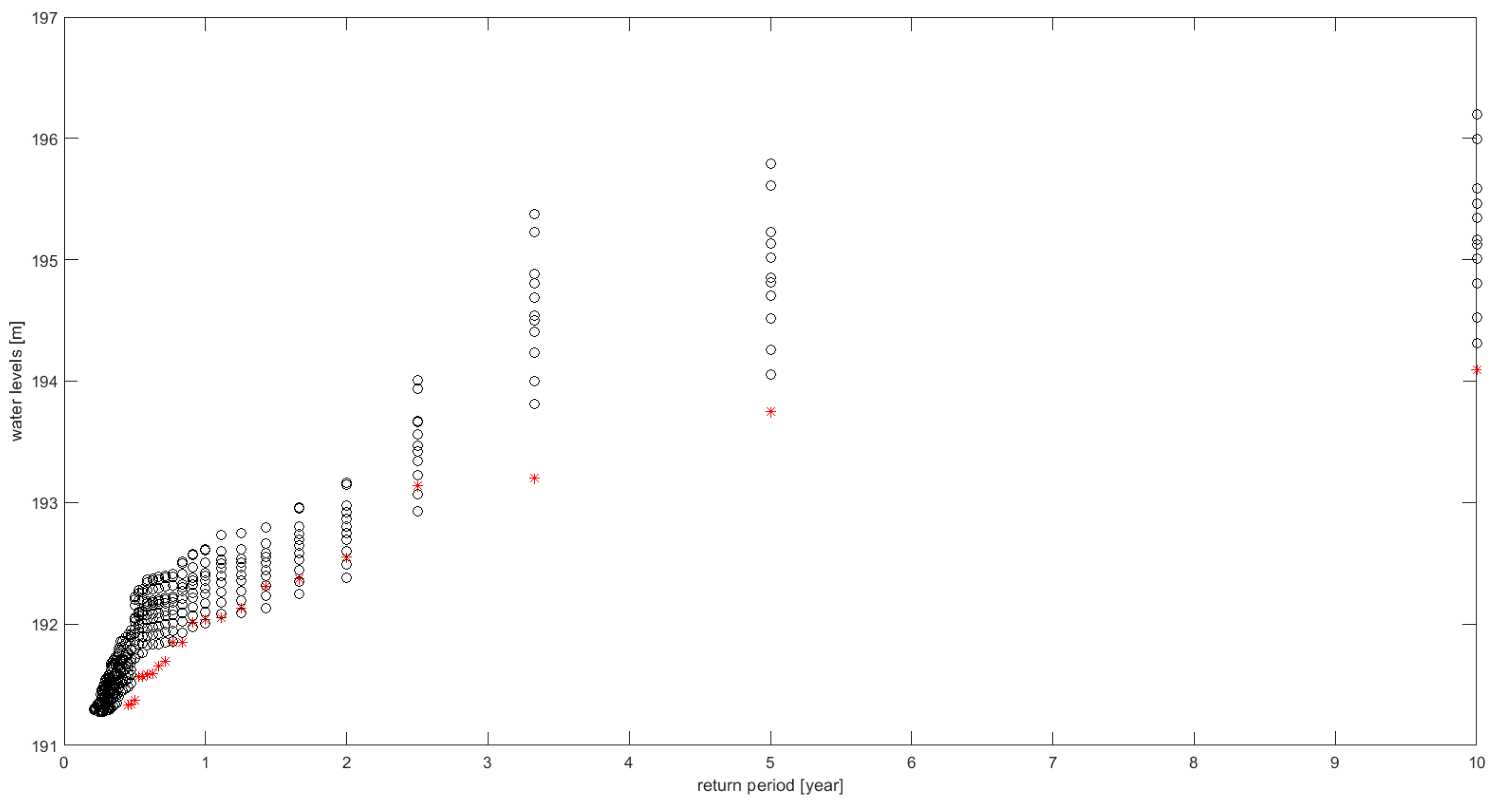
Figure 9 presents an example of an empirical relationship between the return period and water levels obtained for the 10-year long time series of simulated water levels at the Koszyce Wielkie gauging station for the period 1991–2000. The black-marked curves correspond to nine different parameter sets of the Monte–Carlo ensemble simulations, while the red-marked curve is obtained for the observed time series.
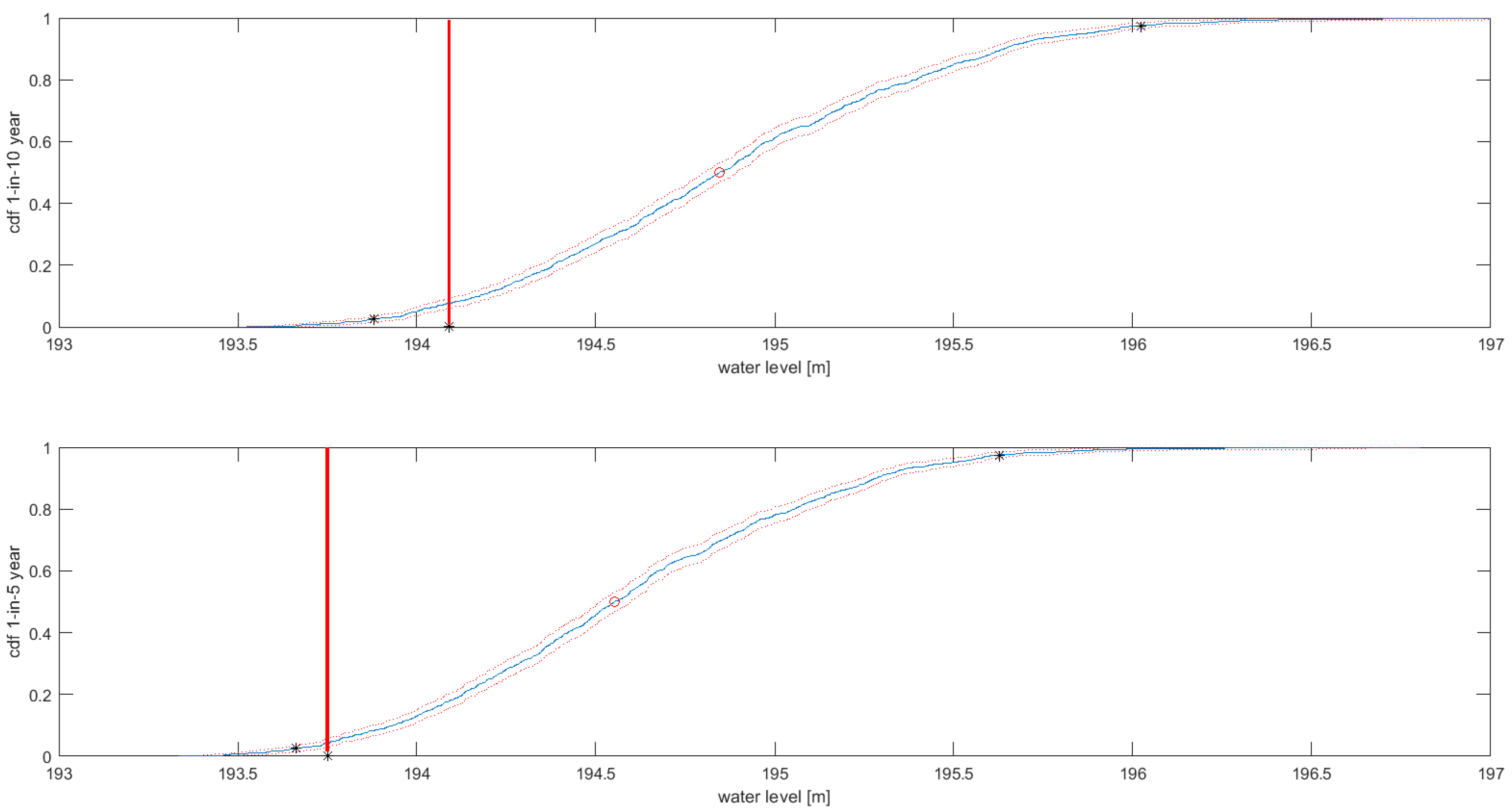
The evaluation of return periods allows for a comparison of the modeling results with the observations for different return periods. Figure 10 presents the derived 1-in-5 and 1-in-10 year return period water levels in the Koszyce gauging station obtained from an MC analysis of emulator predictions. The observations, denoted by red perpendicular lines, indicate slight over-predictions of emulator simulations. The 0.95 confidence bands for the 1-in-10 year return period predictions are about 2 m wide. We noted that the Box–Cox model parameters have the largest influence on the spread of the results and can be used to derive weights describing model goodness of fit. However, those weights are local, i.e., they depend on the local differences between the predicted and modeled water levels and cannot be extrapolated to other sites.
This illustration indicates the importance of observations of inundation extent (water levels) that would allow the uncertainty of the predictions to be reduced.
The resulting water level uncertainty is transposed into the inundation extent uncertainty through the water-level–inundation-extent relationship (right panel of Figure 6). This will result in a different inundation area uncertainty depending on the incoming upstream flow.
3.3. Derivation of Flood Hazard Maps for the Future
The EURO-CORDEX initiative project [41] was used as a source of daily temperature and precipitation projections for the period 1971–2100. The projections have a spatial resolution of 12.5 km (EUR-11) for the RCP4.5 emission scenario. The ensemble applied in this study has seven members, consisting of four different RCMs driven by three different GCMs (Table 4).
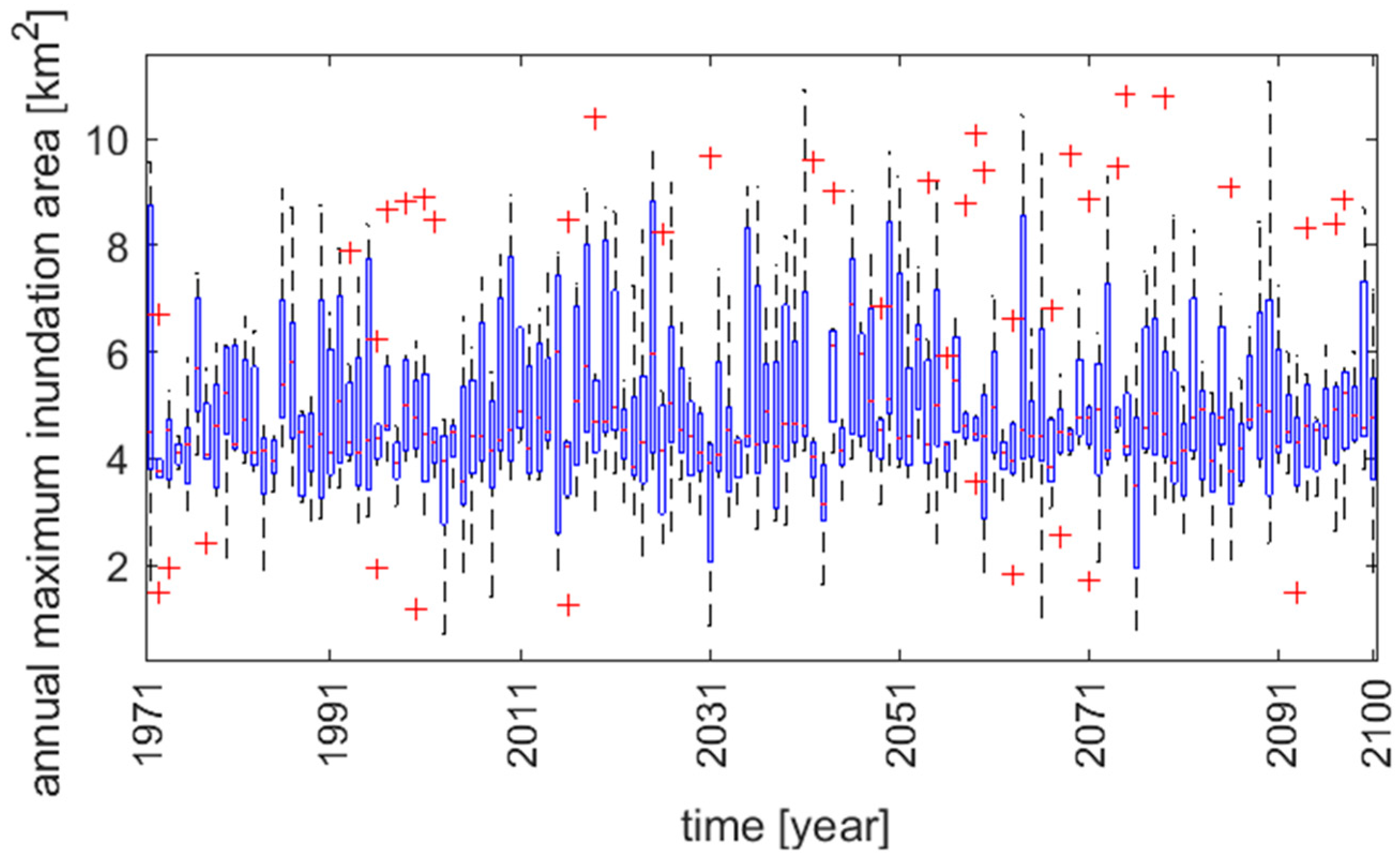
The bias correction of the projected climate variables is usually performed in order to improve their physical interpretability [42]. However, all bias correction methods alter the extreme values, which might be not justified for high flow extremes. Therefore, it was decided to use raw precipitation projections in the present study of projections of maximum flood inundation extent. The simulation procedure described in Section 2 was followed to produce a series of projected annual maximum inundation areas for the Tuchow meander for the seven climate models, for the 1971–2100 period. The results are presented in Figure 11.
The projected maximum annual inundation areas for the seven models show a stationary character, which results from a stationary character of the annual maximum flow projections for the Biala Tarnowska [32]. However, looking at the outliers denoted by red crosses, the increase in annual maximum inundation areas can be found. Closer examination of precipitation projections (not shown here) reveals that 130-year daily raw precipitation data contain peaks of extreme precipitation, which are caused by the regional climate model instability (the so-called one-grid storms). These abnormal events may lead to wrong conclusions on the future projections of extreme high flow events when linear regression models are used to analyze future trends and the uncertainty of the projections is not taken into account [32].
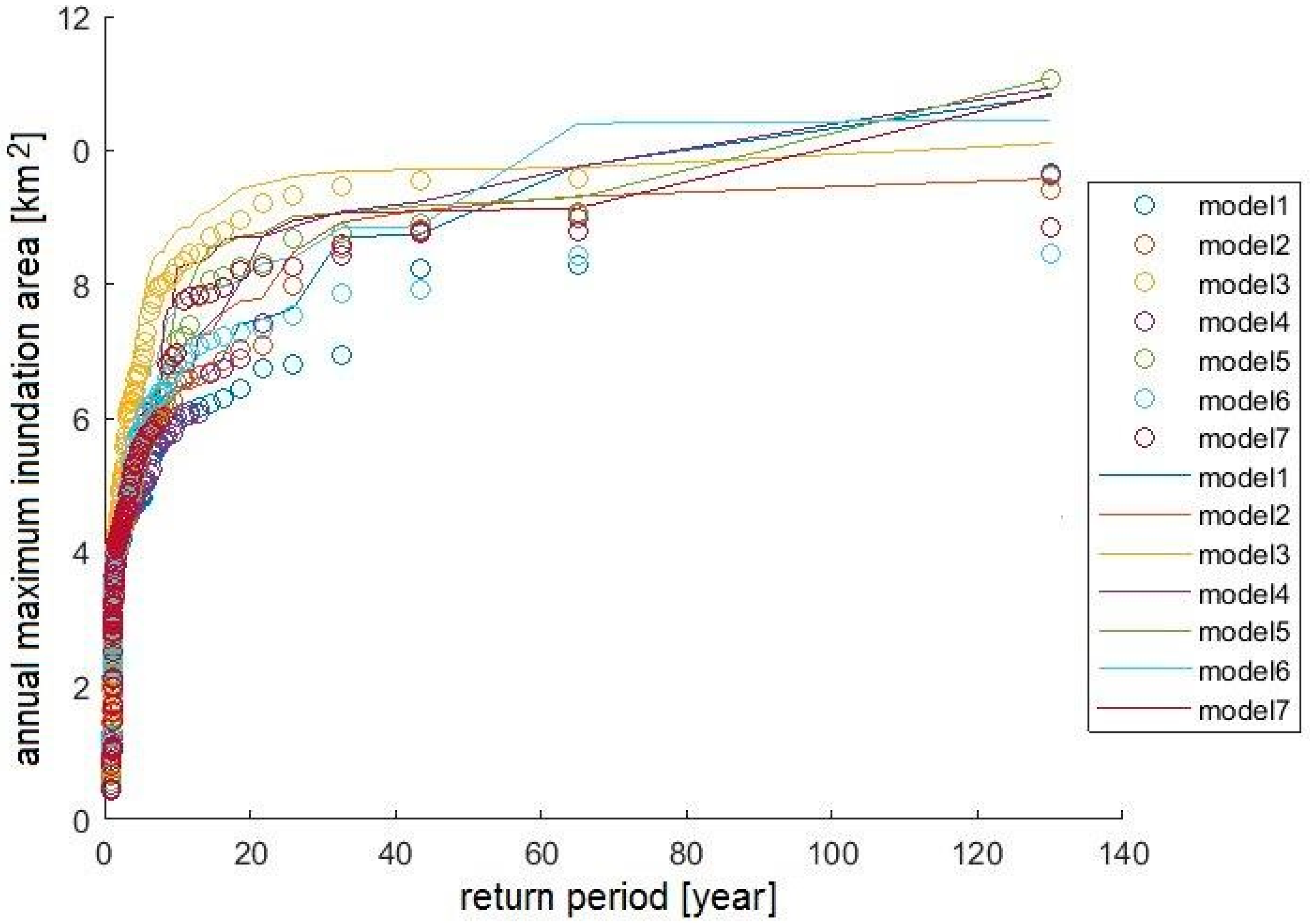
The instabilities were detected by a comparison with the precipitation projections for the neighboring catchment Dunajec. The extreme event should appear in both catchments; otherwise, the extreme event is classified as a one-grid storm and replaced by the second-highest event in the year. In this study, instabilities in all but two models were detected. In the case of Biala Tarnowska, Models 2 and 5 were free of one-grid storms (Figure 12). Significant changes in maximum inundation return periods were found for Models 1, 3, 4, 6 and 7.
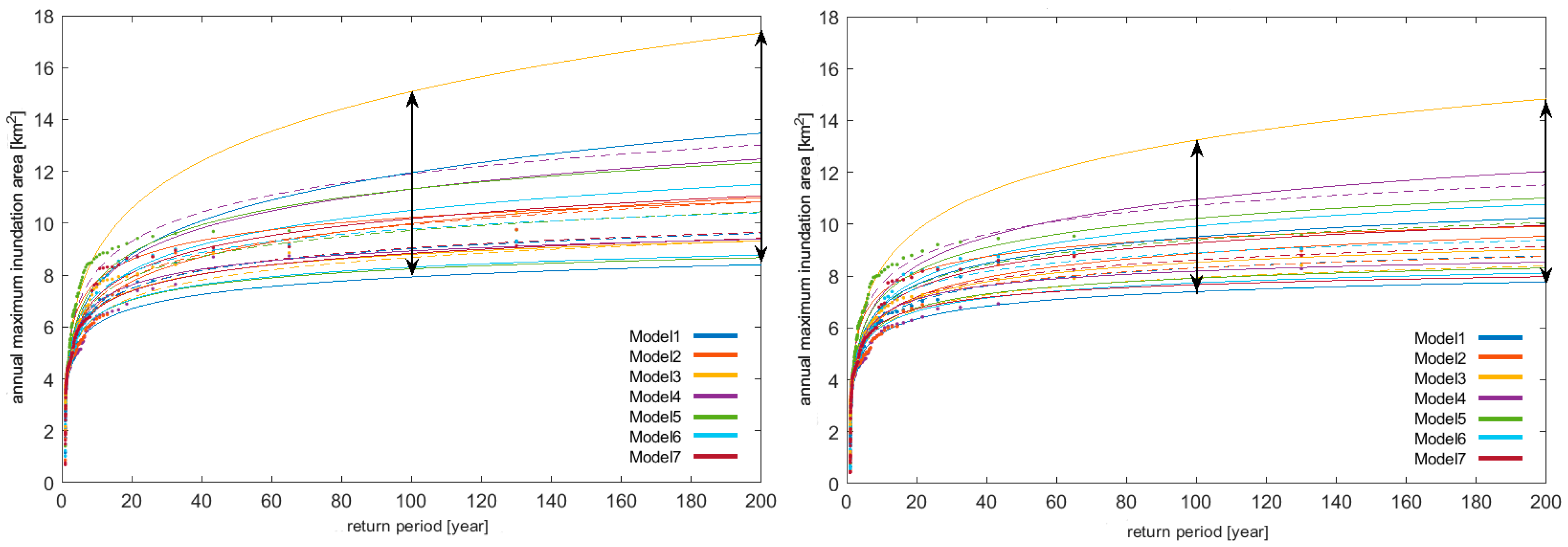
The NEVA routine [43] for the generalized extreme value (GEV) analysis was performed for maximum annual inundation area data presented in Figure 12. The one-grid storms influence the bounds of inundation projection uncertainty (Figure 13). The left panel presents an analysis of data without one-grid storms, while the right panel presents results with one-grid storms. Obviously, the uncertainty bounds are smaller in the case of data without RCM instabilities.
Removing one-grid storm events significantly change the results by decreasing the bounds of uncertainty of the inundation area.
4. Conclusions
The main issue related to the simulation approach within future climate change projections is the simulation time. The size, and above all the amount, of data derived from the projections that have to be processed by a distributed model make flood risk mapping very time-consuming. To accelerate the process, an emulator of a distributed model was applied. The emulator of the 1D MIKE11 was based on a stochastic transfer function that presents linear process dynamics, while the linearization of a flow–water-level relationship was performed with the Box–Cox transformation, which acts as an inverse of a rating curve. The use of the emulator significantly speeds up the process but may cause other problems, related mainly to simplification errors and the difficulty in assessing the uncertainty of its predictions when spatial observations are missing. However, the latter applies also to a distributed flow routing model. The way forward is further work on the development of remote sensing methods, using the unmanned aerial system (UAS) to derive local aerial photographs of the inundation extent.
Using the Tuchow meander as an example, relationships have been derived between the simulated water depth at a given cross section on the meander and the meander inundation area for the annual maximum flows (Figure 6). Those relationships can be used to assess the sensitivity of maximum inundation area to changes in annual maximum flows governed by climatic changes.
An additional advantage of the simulation approach presented here is the taking into account of the variability of antecedent conditions in the catchment before a flood event. The other approach to the derivation of flood risk maps that uses a design storm of a specified return period derived from the precipitation projections [44] results in inundation area projections that are biased and depend on assumed soil moisture conditions before the storm.
There is a large uncertainty in climate projections that influences the estimates of future flood risk. The crucial action in the case of adaptation to floods is a double check of climate projections. We show that the pre-processing of climate projections, by excluding one-grid storms (instabilities), significantly reduces the uncertainty of inundation projections.
Author Contributions
Conceptualization: J.D. and R.J.R.; methodology: J.D. and R.J.R.; software: J.D. and R.J.R. and A.K.; validation: R.J.R.; formal analysis: J.D.; investigation: J.D. and R.J.R.; data curation: J.D.; writing—original draft preparation: J.D. and R.J.R.; writing—review & editing: J.D., R.J.R., and A.K.; visualization: J.D. and R.J.R.; supervision: R.J.R.
Funding
This work was partially supported within statutory activities No 3841/E-41/S/2017 of the Ministry of Science and Higher Education of Poland.
Conflicts of Interest
The authors declare no conflict of interest.
References
- European Flood Directive 2007. Available online: http://ec.europa.eu/environment/water/flood_risk/index.htm (accessed on 27 December 2018).
- Popielarz-Deja, S.; Lesniak, E. Examples of Hydrological Computation for Water-Drainage assessments: Methodology and examples of hydrological evaluations in the case of lack of hydrological observations. In Materialy Pomocnicze—Centralne Biuro Studiow i Projektow Wodnych Melioracji; Centralne Biuro Studiów i Projektów Wodnych Melioracji: Warsaw, Poland, 1971. (In Polish) [Google Scholar]
- Faulkner, D.; Wass, P. Flood estimation by continuous simulation in the Don catchment, South Yorkshire, UK. Water and Environment. J. CIWEM 2007, 19, 78–84. [Google Scholar]
- Falter, D.; Schröter, K.; Dung, NV.; Vorogushyn, S.; Kreibich, H.; Hundecha, Y.; Apel, H.; Merz, B. Spatially coherent flood risk assessment based on long-term continuous simulation with a coupled model chain. J. Hydrol. 2015, 524, 182–193. [Google Scholar] [CrossRef] [Green Version]
- Intergovernmental Panel on Climate Change (IPCC). Climate Change 2014: Impacts, Adaptation, and Vulnerability. Part A: Global and Sectoral Aspects. Contribution of Working Group II to the Fifth Assessment Report of the Intergovernmental Panel on Climate Change; IPCC: Geneva, Switzerland, 2014. [Google Scholar]
- European Environment Agency (EEA). Annual Report 2013 and Environmental Statement 2014; Technical Report; European Environment Agency: Copenhagen, Denmark, 2013. [Google Scholar]
- Tanaka, T.; Tachikawa, Y.; Ichikawa, Y.; Yorozu, K. Impact assessment of upstream flooding on extreme flood frequency analysis by incorporating a flood-inundation model for flood risk assessment. J. Hydrol. 2017, 554, 370–382. [Google Scholar] [CrossRef]
- Doroszkiewicz, J.; Romanowicz, R.J. Guidelines for the adaptation to floods in changing climate. Acta Geophys. 2017, 65, 849–861. [Google Scholar] [CrossRef] [Green Version]
- Apel, H.; Thieken, A.H.; Merz, B.; Blöschl, G. Flood risk assessment and associated uncertainty. Nat. Hazards Earth Syst. Sci. 2004, 4, 295–308. [Google Scholar] [CrossRef] [Green Version]
- Komatina, D.; Branisavljevic, N. Uncertainty Analysis as a Complement to Flood Risk Assessment; Faculty of Civil Engineering University of Belgrade: Beograd, Serbia, 2005; Available online: http://daad.wb.tu-harburg.de/fileadmin/BackUsersResources/Risk/Dejan/UncertaintyAnalysis.pdf (accessed on 25 March 2016).
- Kiczko, A.; Romanowicz, R.J.; Osuch, M.; Karamuz, E. Maximising the usefulness of flood risk assessment for the River Vistula in Warsaw. Nat. Hazards Earth Syst. Sci. 2013, 13, 3443–3455. [Google Scholar] [CrossRef] [Green Version]
- Romanowicz, R.J.; Kiczko, A. An event simulation approach to the assessment of flood level frequencies: Risk maps for the Warsaw reach of the river Vistula. Hydrol. Process. 2016, 30, 2451–2462. [Google Scholar] [CrossRef]
- Castelletti, A.; Galelli, S.; Restelli, M.; Soncini-Sessa, R. Data-driven dynamic emulation modelling for the optimal management of environmental systems. Environ. Model. Softw. 2012, 34, 30–43. [Google Scholar] [CrossRef]
- Merz, B.; Thieken, A.H. Flood risk curves and uncertainty bounds. Nat. Hazards 2009, 51, 437–458. [Google Scholar] [CrossRef] [Green Version]
- Water Act 20 July 2017 r. in Polish, Ustawa z dnia 20 lipca 2017 r. Prawo wodne (Dz.U. z 2017 poz. 1566). Available online: http://prawo.sejm.gov.pl/isap.nsf/DocDetails.xsp?id=WDU20170001566 (accessed on 22 February 2018).
- Jones, R.N. Managing uncertainty in climate change projections—Issues for impacts assessments. Clim. Chang. 2000, 45, 403–419. [Google Scholar] [CrossRef]
- Wilby, R.L.; Suraje, D. Robust adaptation to climate change. Weather 2010, 65, 180–185. [Google Scholar] [CrossRef] [Green Version]
- Chen, I.-C.; Hill, J.K.; Ohlemüller, R.; Roy, D.B.; Thomas, C.D. Rapid range shifts of species associated with high levels of climate warming. Science 2011, 333, 1024–1026. [Google Scholar] [CrossRef] [PubMed]
- Willems, P.; Vrac, M. Statistical precipitation downscaling for small-scale hydrological impact investigations of climate change. J. Hydrol. 2011, 402, 193–205. [Google Scholar] [CrossRef]
- Piani, C.; Weedon, G.P.; Best, M.; Gomes, S.M.; Viterbo, P.; Hagemann, S.; Haerter, J.O. Statistical bias correction of global simulated daily precipitation and temperature for the application of hydrological models. J. Hydrol. 2010, 395, 199–215. [Google Scholar] [CrossRef]
- Osuch, M.; Romanowicz, R.J.; Lawrence, D.; Wong, W.K. Trends in projections of standardized precipitation indices in a future climate in Poland. Hydrol. Earth Syst. Sci. 2016, 20, 1947–1969. [Google Scholar] [CrossRef]
- Romanowicz, R.J.; Kiczko, A.; Napiorkowski, J.J. Stochastic transfer function model applied to combined reservoir management and flow routing. Hydrol. Sci. J. 2010, 55, 27–40. [Google Scholar] [CrossRef] [Green Version]
- Foglia, L.; Hill, M.C.; Mehl, S.W.; Burlando, P. Sensitivity analysis, calibration, and testing of a distributed hydrological model using error-based weighting and one objective function. Water Resour. Res. 2009, 45. [Google Scholar] [CrossRef] [Green Version]
- Romanowicz, R.J.; Bogdanowicz, E.; Debele, S.; Doroszkiewicz, J.; Hisdal, H.; Lawrence, D.; Meresa, H.; Napiorkowski, J.; Osuch, M.; Strupczewski, W.G.; et al. Climate change impact on hydrological extremes: Preliminary results from the Polish-Norwegian project. Acta Geophys. 2016, 64, 477–509. [Google Scholar] [CrossRef]
- Bergstrom, S. The HBV model. In Computer Models in Watershed Hydrology; Singh, V.P., Ed.; Water Resources Publications: Highland Ranch, CO, USA, 1995; pp. 443–476. [Google Scholar]
- Hamon, W.R. Estimating Potential Evapotranspiration. Bachelor’s Thesis, Department of Civil and Sanitary Engineering, Massachusetts Institute of Technology, Cambridge, MA, USA, 1960. [Google Scholar]
- Abbott, M.B.; Bathurst, J.C.; Cunge, J.A.; OConnell, P.E.; Rasmussen, J. An introduction to the European Hydrological System Systeme Hydrologique Europeen, SHE, 1: History and philosophy of a physically-based, distributed modelling system. J. Hydrol. 1986, 87, 45–59. [Google Scholar] [CrossRef]
- Stelling, G.S.; Duinmeijer, S.P.A. A staggered conservative scheme for every Froude number in rapidly varied shallow water flows. Int. J. Numer. Methods Fluids 2003, 43, 1329–1354. [Google Scholar] [CrossRef]
- Barkau, R. UNET, One-Dimensional Flow through a Full Network of Open Channels; User’s Manual Version 2.1; Publication CPD-66; Hydrologic Engineering Center, US Army Corps of Engineers: Davis, CA, USA, 1996. [Google Scholar]
- Cholet, C.; Charlier, J.-B.; Moussa, R.; Steinmann, M.; Denimal, S. Assessing lateral flows and solute transport during floods in a conduit-flow-dominated karst system using the inverse problem for the advectiondiffusion equation. Hydrol. Earth Syst. Sci. 2017, 21, 3635–3653. [Google Scholar] [CrossRef]
- Storn, R.; Price, K.V. Differential Evolution—A Simple and Efficient Adaptive Scheme for Global Optimization Over Continuous Spaces; Technical Report TR-95-012; International Computer Sciences Institute: Berkeley, CA, USA, 1995. [Google Scholar]
- Meresa, H.K.; Romanowicz, R.J. The critical role of uncertainty in projections of hydrological extremes. Hydrol. Earth Syst. Sci. 2017, 21, 4245–4258. [Google Scholar] [CrossRef] [Green Version]
- Young, P.C. Recursive Estimation and Time Series Analysis; Springer-Verlag: Berlin, Germany, 1984. [Google Scholar]
- Romanowicz, R.J.; Young, P.C.; Beven, K.J.; Pappenberger, F. A data based mechanistic approach to nonlinear flood routing and adaptive flood level forecasting. Adv. Water Resour. 2008, 31, 1048–1056. [Google Scholar] [CrossRef]
- Nelder, J.A.; Mead, R. A Simplex Method for Function Minimization. Comput. J. 1965, 7, 308–313. [Google Scholar] [CrossRef]
- Romanowicz, R.J.; Doroszkiewicz, J.M. The Application of Cumulants to Flow Routing. Meteorol. Hydrol. Water Manag. 2018, 7. [Google Scholar] [CrossRef]
- Aronica, G.; Bates, P.D.; Horritt, M.S. Assessing the uncertainty in distributed model predictions using observed binary pattern information within glue. Hydrol. Process. 2002, 16, 2001–2016. [Google Scholar] [CrossRef]
- Horritt, M.S.; Bates, P.D. Predicting floodplain inundation: Raster-based modelling versus the finite-element approach. Hydrol. Process. 2001, 15, 825–842. [Google Scholar] [CrossRef]
- Romanowicz, R.J.; Osuch, M. Assessment of land use and water management induced changes in flow regime of the Upper Narew. Phys. Chem. Earth 2011, 36, 662–672. [Google Scholar] [CrossRef]
- Steenbergen, N.; Willems, P. Method for testing the accuracy of rainfall–runoff models in predicting peak flow changes due to rainfall changes, in a climate changing context. J. Hydrol. 2012, 414–415, 425–434. [Google Scholar] [CrossRef]
- Kotlarski, S.; Keuler, K.; Christensen, O.B.; Colette, A.; Déqué, M.; Gobiet, A.; Goergen, K.; Jacob, D.; Lüthi, D.; van Meijgaard, E.; et al. Regional climate modeling on European scales: A joint standard evaluation of the EURO-CORDEX RCM ensemble. Geosci. Model Dev. 2014, 7, 1297–1333. [Google Scholar] [CrossRef]
- Teutschbein, C.; Seibert, J. Bias correction of regional climate model simulations for hydrological climate-change impact studies: Review and evaluation of different methods. J. Hydrol. 2012, 456–457, 12–29. [Google Scholar] [CrossRef]
- Cheng, L.; AghaKouchak, A.; Gilleland, E.; Katz, R.W. Non-stationary extreme value analysis in a changing climate, climatic change. Clim. Chang. 2014, 127, 353–369. [Google Scholar] [CrossRef]
- Papaioannou, G.; Efstratiadis, A.; Vasiliades, L.; Loukas, A.; Papalexiou, S.; Koukouvinos, A.; Tsoukalas, I.; Kossieris, P. An operational method for flood directive implementation in ungauged urban areas. Hydrology 2018, 5, 24. [Google Scholar] [CrossRef]
Figure 1.
The location of the study catchment; left picture: county scale, whole catchment; right picture: local scale, routing model part.
Figure 1.
The location of the study catchment; left picture: county scale, whole catchment; right picture: local scale, routing model part.

Figure 2.
Scheme of an application of an emulator of MIKE11 for climate projections.

Figure 3.
Module of an emulator based on flow–water-level relationship; denotes flow at the 1st cross section at time , for ; denotes water levels at the cross section at time ; denotes the Box–Cox transformation between flow used as an input at the first cross section and the transfer function input .

Figure 4.
The STF-based MIKE11 emulator of water level predictions; on the Biala Tarnowska River—the meander near Tuchow city.
Figure 4.
The STF-based MIKE11 emulator of water level predictions; on the Biala Tarnowska River—the meander near Tuchow city.

Figure 5.
The STF-based MIKE11 emulator of water level predictions, validation stage, the Ciezkowice–Koszyce Wielkie model. The black dots denote MIKE11 simulations; the continuous black line denotes the emulator predictions; the red line denotes the observed water levels at the Koszyce Wielkie gauging station; the shaded area denotes 0.96 confidence limits.

Figure 6.
Dependence on hydrological input (annual maxima) and routing model predictions for the Tuchow meander for the reference period 1971–2010. (a) Water depth values at the 10th cross section of the meander versus the maximum annual flow; (b) inundation areas at the Tuchow meander versus the maximum annual flow; (c) inundation area versus the maximum annual water depth at the 10th cross section of the Tuchow meander. Blue dots denote the data, and green lines denote the fitted curve to the square polynomial.

Figure 7.
Maximum inundation extent of MIKE11 (blue) and the emulator of MIKE11 (magenta) for the year 1997 for a part of the Tuchow meander, and the CSI-based difference (green).
Figure 7.
Maximum inundation extent of MIKE11 (blue) and the emulator of MIKE11 (magenta) for the year 1997 for a part of the Tuchow meander, and the CSI-based difference (green).

Figure 8.
Classification of high water levels at Koszyce Wielkie gauging station for the threshold value equal to the 75th percentile.
Figure 8.
Classification of high water levels at Koszyce Wielkie gauging station for the threshold value equal to the 75th percentile.

Figure 9.
Example of return-period–water-level relationship for the peak water level ensemble.

Figure 10.
Empirical cumulative distribution function (cdf) of water levels with 1-in-10 year return period (upper panel) and 1-in-5 year return period (lower panel) obtained for the Monte Carlo (MC) simulations of peak water levels at Koszyce Wielkie (blue lines); red dotted lines show the cdf 0.95 confidence bounds; black stars show the 0.025, 0.5, and 0.975 quantiles water levels with 1-in-10 and 1-in-5 year return periods; the observed water levels corresponding to 1-in-10 and 1-in-5 year return periods are shown by the red lines.

Figure 11.
Maximum annual inundation from Models 1–7. Median: red lines in the boxes. The bottom and top edges of the blue box indicate the 25th and 75th percentiles, respectively. Maximum and minimum values: dashed black line in each box; red ‘+’: outliers.
Figure 11.
Maximum annual inundation from Models 1–7. Median: red lines in the boxes. The bottom and top edges of the blue box indicate the 25th and 75th percentiles, respectively. Maximum and minimum values: dashed black line in each box; red ‘+’: outliers.

Figure 12.
Return period for 130 annual maxima of inundation area for seven models without a one-grid-storm (‘o’) and with a one-grid-storm (solid line).
Figure 12.
Return period for 130 annual maxima of inundation area for seven models without a one-grid-storm (‘o’) and with a one-grid-storm (solid line).

Figure 13.
Annual maximum inundation area over a 100-year return period (marked with a black double arrow) and a 200-year return period (marked with a black double arrow), with instabilities (left plot) and without instabilities (right plot), the 95% and 5% confidence bounds (respectively with the Models, solid colorful lines), and MLE (dashed lines).


Table 1.
The HBV model parameter values for the Biala catchment, Ciezkowice and Koszyce Wielkie.
| HBV Routines | Name of the Parameter | Ciezkowice | Koszyce Wielkie | Unit |
|---|---|---|---|---|
| soil routine | P.FC | 61.19 | 119.55 | mm |
| P.BETA | 1.68 | 2.89 | non | |
| P.LP | 1 | 1 | non | |
| P.CFLUX | 0.6 | 0.23 | mm/day | |
| surface water balance routine | P.ALFA | 0.24 | 0.27 | non |
| P.KF | 0.3 | 0.11 | day | |
| P.KS | 0.11 | 1.64 | day | |
| soil moisture routine | P.PERC | 1.33 | 1.12 | mm/day |
| snow routine | O.TT | 1.23 | 1.05 | °C |
| O.TTI | 4.93 | 7 | °C | |
| O.FOCFMAX/DTTM | 0.01 | 1.36 | °C/mm day | |
| O.CFMAX | 1.27 | 1.00 | °C/mm day | |
| O.CFR | 0.71 | 0.00 | non | |
| O.WHC | 0 | 0 | mm/mm |
Table 2.
Time processing for the 1971–2010 period and an area of 42 km2.
| Time of Processing | Map Based on MIKE11 Results (s) | Map Based on the Emulator of MIKE11 Results (s) |
|---|---|---|
| Routing | 19,035 | 147 |
| calculating a flooded area and saving the inundation map based on 1 m × 1 m resolution DTM | 990 | 990 |
| TOTAL | 20,015 (≈5 h 34 min) | 1137 (≈19 min) |
Table 3.
Parameter values of the emulator of the MIKE11 Ciezkowice–Koszyce Wielkie model and their uncertainty. Parameters are defined by Equations (1) and (2), where P/R denotes the cross-correlation between P and R.
Table 3.
Parameter values of the emulator of the MIKE11 Ciezkowice–Koszyce Wielkie model and their uncertainty. Parameters are defined by Equations (1) and (2), where P/R denotes the cross-correlation between P and R.
| Parameter [Unit] | Mean | Variance |
|---|---|---|
| P [-] | 0.8710 | 0.1943 × 10⁻⁶ |
| R [-] | 0.0199 | 0.0045 × 10⁻⁶ |
| P/R [-] | - | 0.029 × 10⁻⁶ |
| δ [h] | 13 | 0 |
| c [-] | −0.2740 | 0.03 |
| b [-] | 0.5246 | 0.03 |
| ε [-] | 0 | 0.008 |
Table 4.
List of RCM/GCMs used in this study.
| Model Number | GCM | RCM | Full Name | Source Institution |
|---|---|---|---|---|
| 1 | EC-EARTH | RCA | Rossby Center regional | Swedish Meteorological and Hydrological Institute |
| 2 | EC-EARTH | HIRHAM | Not applicable | Danish Meteorological Institute |
| 3 | EC-EARTH | CCLM | Community Land Model | Not applicable |
| 4 | EC-EARTH | RACMO | Regional Atmospheric Climate Model | Not applicable |
| 5 | MPI | CCLM | Community Land Model | Not applicable |
| 6 | MPI | REMO | Regional-scale Model | Max Planck Institute for Meteorology |
| 7 | CNRM | CCLM | Community Land Model | CERFACS, France |
© 2018 by the authors. Licensee MDPI, Basel, Switzerland. This article is an open access article distributed under the terms and conditions of the Creative Commons Attribution (CC BY) license (http://creativecommons.org/licenses/by/4.0/).
Share and Cite
MDPI and ACS Style
Doroszkiewicz, J.; Romanowicz, R.J.; Kiczko, A. The Influence of Flow Projection Errors on Flood Hazard Estimates in Future Climate Conditions. Water 2019, 11, 49. https://doi.org/10.3390/w11010049
AMA Style
Doroszkiewicz J, Romanowicz RJ, Kiczko A. The Influence of Flow Projection Errors on Flood Hazard Estimates in Future Climate Conditions. Water. 2019; 11(1):49. https://doi.org/10.3390/w11010049
Chicago/Turabian StyleDoroszkiewicz, Joanna, Renata J. Romanowicz, and Adam Kiczko. 2019. "The Influence of Flow Projection Errors on Flood Hazard Estimates in Future Climate Conditions" Water 11, no. 1: 49. https://doi.org/10.3390/w11010049
Note that from the first issue of 2016, this journal uses article numbers instead of page numbers. See further details here.