Heavy Metals in Bottom Sediments of Reservoirs in the Lowland Area of Western Poland: Concentrations, Distribution, Sources and Ecological Risk


1
Institute of Land Improvement, Environmental Development and Geodesy, Poznań University of Life Sciences, Piątkowska 94, 60-649 Poznań, Poland
2
Department of Hydrogeology and Water Protection, Institute of Geology, Adam Mickiewicz University, 12 Bogumiła Krygowskiego Street, 61-680 Poznań, Poland
*
Author to whom correspondence should be addressed.
Water 2019, 11(1), 56; https://doi.org/10.3390/w11010056
Submission received: 6 November 2018
/
Revised: 5 December 2018
/
Accepted: 25 December 2018
/
Published: 31 December 2018
(This article belongs to the Section Water Quality and Contamination)
Abstract
:The paper presents the results of a study of heavy metals (HMs) concentrations in six retention reservoirs located in the lowland area of western Poland. The objectives of this study were to analyze the Cd, Cr, Cu, Ni, Pb and Zn concentrations, assess contamination and ecological risk, analyze the spatial variability of HM concentrations and identify potential sources and factors determining the concentration and spatial distribution. The bottom sediment pollution by HMs was assessed on the basis of the index of geo-accumulation (Igeo), enrichment factor (EF), pollution load index (PLI) and metal pollution index (MPI). To assess the ecological risk associated with multiple HMs, the mean probable effect concentration (PEC) quotient (Qm-PEC) and the toxic risk index (TRI) were used. In order to determine the similarities and differences between sampling sites in regard to the HM concentration, cluster analysis (CA) was applied. Principal component analysis (PCA) was performed to assess the impact of grain size, total organic matter (TOM) content and sampling site location on HM spatial distribution. Additionally, PCA was used to assess the impact of catchment, reservoir characteristics and hydrological conditions. The values of Igeo, EF, MPI and PLI show that Cd, Cr, Cu, Ni and Pb mainly originate from geogenic sources. In contrast, Zn concentrations come from point sources related to agriculture. The mean PEC quotient (Qm-PEC) and TRI value show that the greatest ecological risk occurred at the inlet to the reservoir and near the dam. The analysis showed that the HMs concentration depends on silt and sand content. However, the Pb, Cu, Cd and Zn concentrations are associated with TOM as well. The relationship between individual HMs and silt was stronger than with TOM. The PCA results indicate that HMs with the exception of Zn originate from geogenic sources—weathering of rock material. However, the Ni concentration may additionally depend on road traffic. The results show that a reservoir with more frequent water exchange has higher HMs concentrations, whereas the Zn concentration in bottom sediments is associated with agricultural point sources.
1. Introduction
Reservoirs play important roles in water supply, irrigation, power generation and flood control. However, dam construction changes the hydrological regime and sediment transport [1,2,3]. The suspended sediments are stored in the reservoir and with them pollutants including heavy metals (HMs) [4]. Bottom sediment plays an important role in monitoring the aquatic environment [5], especially evaluating the contamination levels [6,7], and ecological risk assessment [8].
HMs have natural, i.e., geogenic (weathering and erosion), and anthropogenic origin (urban domestic and industrial waste and the use of chemical fertilizers, roadside soil) [5,7,9,10,11]. They are classified as serious environmental pollutants due to persistence, tendency to bioaccumulate and high toxicity [12].
The spatial distribution in HM concentrations among reservoirs is associated with different anthropogenic activities [13,14]. The distribution depends on hydrodynamic conditions, type of sediment and metal sources [15]. Moreover, shape and morphology of the reservoir [16], reservoir operation [17] and the biochemical processes [18] modify the HM deposition. The highest concentrations have been detected generally in the vicinity of polluted water inflow [10]. River-reservoir interaction might modify the impact of HM point sources [19]. Intensified accumulation of sediments and pollutants has been observed especially in the vicinity of dams [17,20]. The concentrations of HMs in bottom sediments varied in different sampling locations and layers, but the concentrations in the surface layer are higher than those in the deeper layers [21]. Generally, the concentration of HMs was higher in reservoir sediments than in river sediments [16,22]. However, Frémion et al. [23] indicated that the HM concentrations are lower in the reservoir than upstream and downstream, which is caused by the high fresh organic matter inputs, diluting the contamination. Seasonal variations of metal concentrations depend on hydrological conditions, the impact of non-point sources and lithogenic sources [24].
The distribution of HMs in the sediments was mainly connected with grain size and organic matter content [25,26]. Fine-grain sediments contain higher HM concentrations [27], which is related to higher magnetic susceptibility [8]. Farhat and Aly [28] suggested that the organic matter was more important in controlling HM distribution. Organic matter was a key mediator for ecological risk [29]. Metals released into reservoirs are generally bound to the sediment bottom [30,31]. However, HMs may be released into the water column via sediment resuspension, due to changing chemical and hydrological conditions [23,32,33,34,35] and accumulate in plants and animals [2,26,36,37]. Higher concentrations of HMs can cause toxicity risk to the biota and human health [38,39,40,41]. Birch and Apostolatos [42] showed that anthropogenic metals have higher mobility and bioavailability than metals from geogenic origin.
Flow regulation, local geomorphological characteristics and reservoir operations determine the redistribution of HMs [39,43]. In dam reservoirs the water-level fluctuation zone is important for the accumulation and redistribution of HMs [29,44]. Moreover, dredging operations, the emptying of reservoirs and flood events might lead to release of HMs to the water environment [45,46,47,48].
The transport and enrichment of HMs in reservoir bottom sediments have been intensively studied, including concentration, spatial distribution, source identification and pollution assessment [13,49,50,51], temporal variability [52], bioavailability [53], ecological risk and organism toxicity [4,54,55]. Moreover, some studies relate to HM concentrations in reservoir tributaries [16,56]. Many methods have been used for the assessment of bottom sediment HM pollution and to determine the potential risk of heavy metal contamination [29,57,58,59,60,61,62,63,64,65,66,67,68,69,70,71].
However, for the assessment of spatial distribution, identification of pollution sources and factors affecting their content in bottom sediments, multivariate statistical have been used [7,26,71,72,73,74,75,76].
Despite the numerous research results available, there are some deficiencies that still need attention. The studies usually focus on a certain reservoir, and less information is available about the HMs’ variation in a group of reservoirs [14]. There is little information available about heavy metal pollution in reservoirs and their changes after prolonged exploitation [77]. Moreover, Wu et al. [78] suggested that future climate change will aggravate the ecological risk of HMs in the water environment due to the release of HMs from sediments to the water environment.
Poland is characterized by high seasonal and spatial variability of water resources. Therefore, in order to increase the efficiency of water management and ensure flood protection, retention reservoirs have been constructed for over 50 years. The largest number of retention reservoirs were constructed in lowland areas of Poland. Their location in the agricultural landscape means that they are exposed to a high supply of nitrogen and phosphorus [79,80,81]. In the reservoirs, seasonal algal blooms and an overgrowing process are observed [82,83,84]. Studies conducted by Baran et al. [85], Wiatkowski [86] and Kasperek and Wiatkowski [87] show that the heavy metal concentrations in reservoir bottom sediments vary across Poland. Concentrations of heavy metals in bottom sediments depend on the catchment land use and the occurrence of pollution point sources [25,88,89]. Therefore, each reservoir should be considered individually in order to expose the factors affecting the bottom sediment pollution. In this study, six reservoirs located in the lowland area of western Poland were selected for analysis. Their selection was influenced by the time of their construction, different morphometric parameters, catchment land use and hydrological conditions. The objectives of this study are to: (1) analyze the concentrations of HMs in bottom sediments, (2) show the spatial variability of heavy metal concentrations, (3) analyze the bottom sediment contamination, (4) assess ecological risk, (5) identify potential sources and factors determining the content and spatial distribution of HMs in the reservoirs.
2. Materials and Methods
2.1. Study Area and Sampling Sites
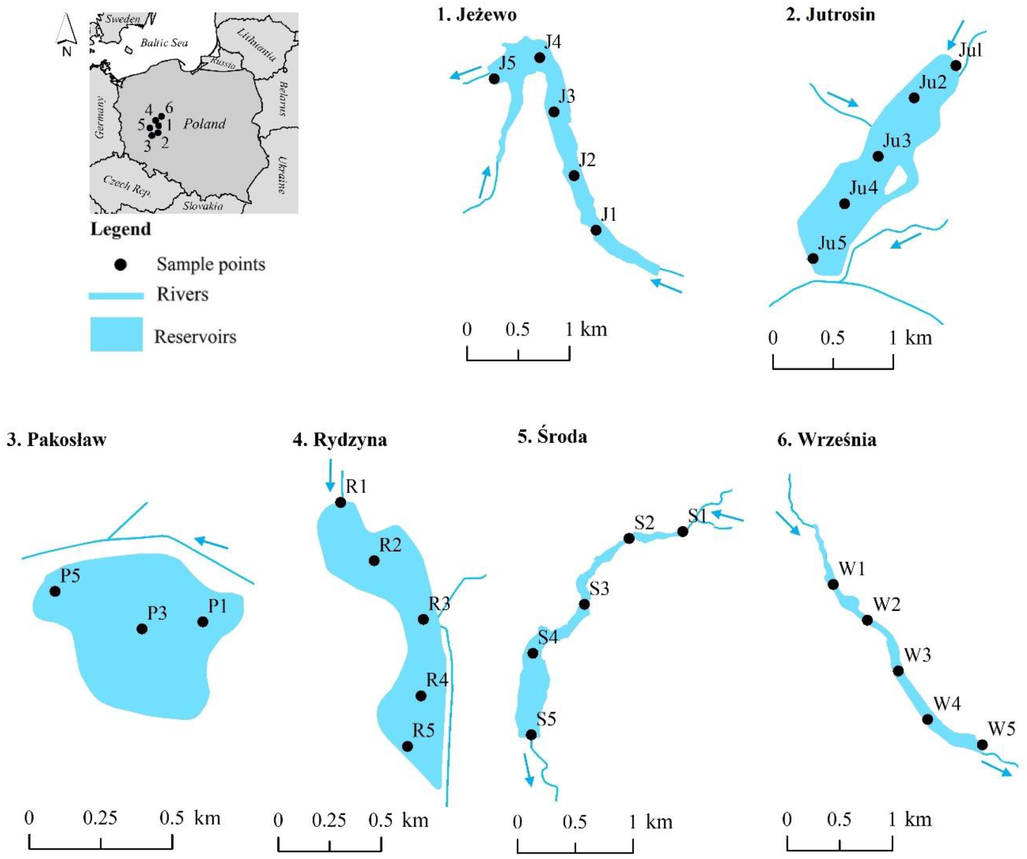
The research was carried out on the example of six reservoirs located in lowland areas in western Poland (Figure 1).
The reservoirs are located in the areas most vulnerable to drought in Poland [90]. The main functions of the reservoirs are to provide water for irrigation purposes. The reservoirs were built between 1967 and 2013 (Table 1). Their surface area ranges from 33 to 91 ha and their volume from 0.3 to 2.4 million m3. They are shallow reservoirs with mean depths ranging from 1.3 to 2.1 m. The greatest depths from 3.5 to 5.5 m are found near the dam. The reservoirs Jeżewo, Jutrosin, Rydzyna, Środa and Września have an elongated shape and their shoreline development ranges from 1.6 to 2.9. However, the Pakosław reservoir has a rounded shape and the shoreline development is 0.8. In the catchment land use structure, agriculture area dominates, its percentage ranging from 68 to 81%. The proportion of urban and industrial areas is small and ranges from 2 to 7% in the Środa, Rydzyna and Jutrosin catchments, respectively. The stream and road density in the catchment range from 1.2 to 2.3 km·km−2 and from 0.9 to 1.1 km·km−2 respectively. The number of river and road crossings where HM inflow may occur ranges from 0.5 to 0.8 no.·km−2.
2.2. Sample Collection and Preparation
The sampling and field surveys took place during September 2017. The total 28 surface sediment samples were collected from six reservoirs (Figure 1). The sampling locations were recorded using a hand-held Global Positioning System (GPS) device (GARMIN OREGON 300). Due to the elongated shape of the Jeżewo, Jutrosin, Radzyny, Środa and Września reservoirs, five samples were taken along the potential flow path. In the case of the Pakosław reservoir, with a rounded shape, three samples were taken. The top 0–5 cm depth of sediment samples was manually collected by means of Nurek and Czapla devices and carried within zip-mouthed PVC packages. In the laboratory, the bottom sediment samples were subjected to grain size and total organic matter (TOM) analysis. The analysis was carried out in order to examine the relationship between bottom sediment characteristics and total HM concentration. In the first step the bottom sediment samples were air dried at room temperature and sieved through a 2 mm nylon sieve to remove coarse debris. Next the samples were homogenized and passed through 2 mm, 1 mm, 0.5 mm, 0.25 mm, 0.10 mm and 0.05 mm sieves. The analysis was done by means of an analytical sieve shaker (Model, AS 200). The grain size fraction less than 0.05 mm was determined according to the Casagrande aerometric method modified by Prószyński [91]. The sand (0.05–2.0 mm), silt (0.002–0.05 mm), and clay (<0.002 mm) fractions were determined. The total organic matter (TOM) was measured by the Tiurin method with wet oxidation, followed by ferrous ammonium sulfate titration [91]. Finally, the samples were prepared for chemical analysis. The bottom sediment samples were extracted with hydrochloric acid (Merck, Darmstadt, Germany) at a 1:4 ratio at 95 °C ± 5 °C in a Mars 5 Xpress microwave digestion system (CEM, Matthews, NC, USA).
2.3. Chemical Analysis
The concentrations of Cd, Cr, Cu, Pb, Ni, and Zn in the bottom sediment samples with a fraction of <2 mm were determined by inductively coupled plasma mass spectrometry (ICP-QQQ), model 8800 Triple Quad (Agilent Technologies Tokyo, Japan). The analytical procedure is described in previous papers [16,73,75]. The reagents used were analytically pure, and the water was purified to the resistivity of 18.2 MΩ·cm (at 25 °C) in a Direct-Q 3 Ultrapure Water Systems apparatus (Millipore Molsheim, France). During the determinations by the ICP-QQQ techniques, standard solutions produced by VHG Labs, Inc. (Manchester, UK) were used. We measured the Certified Reference Material CRM no. LGC 6187 used for River sediments (Manchester, UK), and high compliance with reference values was found.
2.4. Quantification of Metal Pollution
The assessment of bottom sediment pollution by HMs was performed on the basis of four indices: the index of geo-accumulation (Igeo), the enrichment factor (EF) index, the pollution load index (PLI), and the metal pollution index (MPI). Igeo and EF are single indices, while PLI and MPI are integrated indices.
2.4.1. Index of Geo-Accumulation
The index of geo-accumulation Igeo was determined by the equation proposed by Müller [92] as follows (1):
Igeo is a single factor pollution index where Cn and Bn are the concentration of the selected HMs in bottom sediments and the geochemical background value, respectively (mg.kg−1). The factor 1.5 is used for the possible variability of the background data due to lithological conditions. Values of Igeo were used to classify sediment samples into 7 purity classes: class 0 (Igeo ≤ 0)—uncontaminated, class 1 (0 < Igeo ≤ 1)—uncontaminated to moderately contaminated, class 2 (1 < Igeo ≤ 2)—moderately contaminated, class 3 (2 < Igeo ≤ 3)—moderately to heavily contaminated, class 4 (3 < Igeo ≤ 4)—highly contaminated, class 5 (4 < Igeo ≤ 5)—heavily to extremely contaminated, class 6 (5 < Igeo)—extremely contaminated [64].
2.4.2. Enrichment Factor
The enrichment factor (EF) is an efficient index for quantification of the human impact on the concentration of a given metal [93]. The EF is based on a ratio of measured metal concentration to the metal geochemical background value. To account for natural heavy metal concentrations, EF is normalized to sediment Al or Fe content. In this study the normalization with Fe was selected, as proposed by Deely and Fergusson [94]. The EF was calculated as follows [95] (2):
where (Cn/CFe) is the ratio of the concentration of heavy metal (Cn) to iron (CFe) in the sediment sample and (Bn/BFe) is the same ratio for the geochemical background [96,97]. Values of EF were used to assess the pollution of bottom sediment samples into the following classes: 0 (EF ≤ 1) no enrichment; 1 (1 < EF ≤ 3) is minor enrichment; 2 (3 < EF ≤ 5) is moderate enrichment; 3 (5 < EF ≤ 10) is moderately severe enrichment; 4 (10 < EF ≤ 25) is severe enrichment; 5 (25 < EF ≤ 50) is very severe enrichment; and 6 (EF > 50) is extremely severe enrichment [98,99].
2.4.3. Pollution Load Index
The pollution load index (PLI) is an experimental formula developed by Tomlinson et al. [100] (3):
where Cn/Bn is the ratio of selected elements to their background values and i is the number of elements. The empirical index provides simple comparisons of site average heavy metal pollution. PLI value = 0 denotes perfection, PLI < 1 denotes no pollution, and PLI > 1 indicates pollution [101].
2.4.4. Metal Pollution Index
The metal pollution index (MPI) was also used to compare the total metal content between different sampling sites within reservoirs. The MPI was calculated as follows (4):
where Cn are concentrations of HMs in the sample and i is the number of analyzed metals [96,102]. The background heavy metal concentrations in the study area were provided by Bojakowska and Sokołowska [103]. The geochemical background values for bottom sediments were as follows 1.0 for Cd, 10.0 for Cu, 10.0 for Cr, 10.0 for Ni, 25.0 for Pb, 100.0 for Zn and 10,000.0 mg·kg−1 for Fe.
2.5. Ecological Risk Assessment
A consensus-based sediment quality guideline (SQG) was introduced by Macdonald et al. [104] to predict the toxicity of a sediment samples. For each chemical contaminant there are two consensus-based values—threshold effect concentration (TEC) and probable effect concentration (PEC). The concentration of chemical contaminant below the TEC means that undesirable effects are not expected to occur, while above the PEC adverse effects are expected to occur more often than not [39,105,106]. To assess the effects of multiple HMs, the mean PEC quotient (Qm-PEC) was proposed, which can be calculated using Equation (5):
where n is the number of HMs, Cn is the measured concentration of a heavy metal and PECn is the corresponding PEC. The PEC benchmark values for Cd, Cr, Cu, Ni, Pb and Zn are 4.98, 111, 149, 48.6, 128, and 459 mg·kg−1, respectively. The categories for Qm-PEC are classified as: not toxic (Qm-PEC < 0.5) and toxic (Qm-PEC > 0.5).
The toxic risk index (TRI) was developed by Zhang et al. [107] to assess the toxic risk for certain HMs in sediment samples. The TRI is based on threshold (TEL) and probable (PEL) level effects [108]; it can be calculated using Equation (6):
To assess integrated risk of multiple HMs, the TRI can be calculated using Equation (7):
where n is the number of HMs, Ci is the content of each heavy metal in the sediment sample, and TRIi is the toxic risk index of each heavy metal. Five categories of the TRI are classified as: no toxic risk (TRI ≤ 5), low (5 < TRI ≤ 10), moderate (10 < TRI ≤ 15), considerable (15 < TRI ≤ 20), and very high (TRI > 20) [43].
2.6. Distribution and Source Identification
In order to determine the similarities and differences between sampling sites in regard to the HM concentration, cluster analysis (CA) was applied. The CA was carried out using the Ward method with square Euclidean distance as a measure of similarity between clusters. Groups and subgroups were distinguished using the cut-off criteria of 66% and 25% respectively [109]. For the purpose of comparison of HM concentrations between sample sites, the non-parametric Kruskal-Wallis test (K-W, p ≤ 0.05) followed by Dunn’s test as a post-hoc procedure was used. The K-W test was used for verification of the hypothesis of significance of differences between concentrations of HMs in distinguished groups.
Subsequently, to choose the appropriate ordination methods for future analysis, detrended component analysis (DCA) was conducted. The obtained gradients of the first axis of the DCA were shorter than 3.0 SD, which indicates that the HMs were in linear distribution. Glińska-Lewczuk et al. [110] recommended in such cases principal component analysis (PCA). PCA was employed to identify a potential source of HMs and factors that have the greatest impact on their concentration and spatial distribution. The PCA analysis was done in two variants. First the impact of grain size, total organic matter content and sampling site location on HMs’ spatial distribution was evaluated. The percentage content of sand (SA), silt (SI), clay (CL) and total organic matter (TOM) was calculated for each sample. In addition, the distance between sampling site location with respect to inlet (ID) and outlet (OD) of the reservoir was calculated. Second, the impact of other factors was analyzed. The following factors were distinguished: catchment characteristics (catchment area—CA, mean slope—MS, mean elevation—ME, urban and industrial—UI, agriculture—A, forest—F, stream density—DD, road density—RD, number of road and river crossings—RRC), reservoir characteristics (age—AG, area—AR, mean depth—MD, volume—VO, shoreline development—SD), and hydrological conditions (retention time—RT). The above factors were referred to the mean HM concentration in the samples located in the reservoir (J, Ju, P, R, S, W). Before starting the PCA analysis the factors were tested in the context of the occurrence of outliers. The analysis was performed using the two-sided Grubbs test at the significance level of 0.05. Subsequently the HM concentration and factors that may have an impact on HM content and distribution were log-transformed to obtain a normal distribution. In order to avoid misclassification due to differences in data dimensionality, multivariate statistical techniques were applied on standardized data through z-scale transformation [73,74]. The significant principal components were selected based on a Kaiser criterion with eigenvalues higher than 1. The correlation between principal components and analyzed data was classified according to the Liu et al. [111] criterion where values >0.75, 0.75–0.50, and 0.50–0.30 show a strong, moderate and weak relationship, respectively. CA and PCA were conducted using Statistica 13.1 and Canoco 5.0 respectively.
3. Results
3.1. Heavy Metal Content
The characteristic concentrations of HMs (Cd, Cr, Cu, Ni, Pb and Zn) in bottom sediments from 28 sites are shown in Table 2. Generally, the mean concentrations of HMs in reservoirs follow a descending order of Zn > Pb > Cu > Cr > Ni > Cd. The Zn average concentration in reservoirs’ bottom sediments was 452.2 mg·kg−1. The lowest Zn concentrations occurred in the Jutrosin and the highest in the Jeżewo reservoir, 23.1 and 903.7 mg·kg−1 respectively. It was observed that in the Jeżewo, Rydzyna, Środa and Września reservoirs, Zn concentrations higher than 1000 mg·kg−1 were observed at the inlet to the reservoir or near the dam. Pb concentrations at the highest level were in the Jeżewo reservoir (average 17.6 mg·kg−1), while the lowest values were observed in Pakosław (average 2.6 mg·kg−1). A similar tendency was observed in the case of Cu, Cr and Ni concentrations. The average concentrations of Cu, Cr and Ni in the Pakosław reservoir were at a similar level and was on average 2.0 mg·kg−1. In the Jeżewo reservoir, the average concentrations of these elements in bottom sediments were 3 to 5 times higher. The Cd concentrations in the reservoirs were the lowest and ranged from 0.01 to 0.72 mg·kg−1. In the Września reservoir, the average concentration of Cd was about seven times higher than in the Pakosław reservoir. It was observed that Zn concentrations are characterized by the highest variability between the sampling sites and reservoirs; however, Cr concentrations have the lowest variability. The non-parametric Kruskal-Wallis test showed significant differences in Cd, Cu, Zn and Pb concentrations between bottom sediments at individual reservoirs. Differences were not significant only for Cr and Ni concentrations.
3.2. Bottom Sediment Pollution Assessment
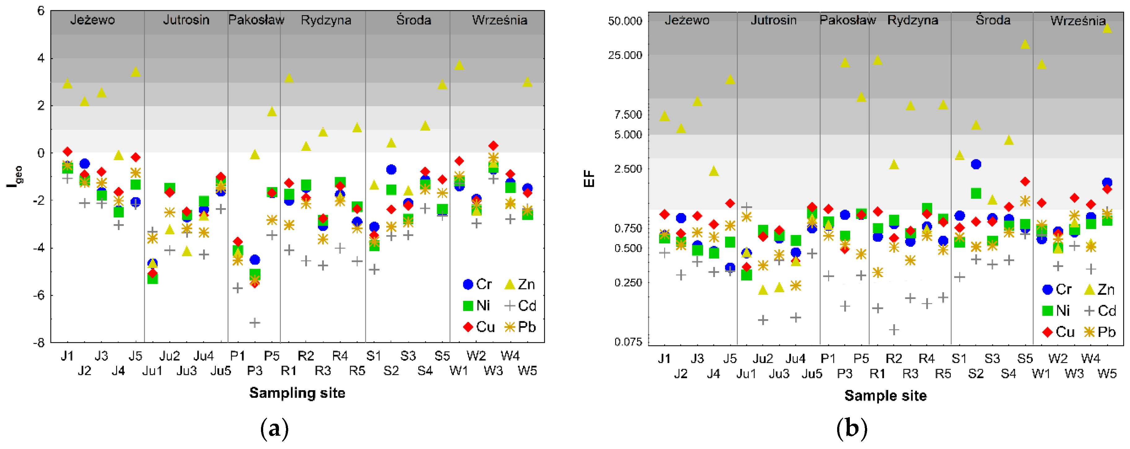
The Igeo was applied to assess the HM contamination level in bottom sediments. The Igeo values for Cd, Cr, Pb and Ni were below zero and could be classified as unpolluted to moderately polluted. The Igeo values for Cu were also lower than 0 except for two sampling sites, J1 and W3. At these points, Igeo values were slightly higher than 0, which indicates a small local contamination of bottom sediments with Cu. The largest contamination of Zn was noted in the reservoirs. Igeo values for Zn lower than 0 occurred only for the Jutrosin reservoir. In 23 measurement sampling sites located in other reservoirs, Igeo values higher than 0 were recorded fourteen times. The sediment bottom at sample sites R2, R3 and S2 demonstrates weak contamination. The values of Igeo were slightly higher than 0. The sediments in sampling sites P5, R5 and S4 demonstrate moderate contamination with the value of Igeo higher than 1. The Igeo for sampling sites J1, J2, J3, J5, R1, S5, W1 and W5 was between 2 and 4, which demonstrated moderate to severe pollution of bottom sediments (Figure 2a).
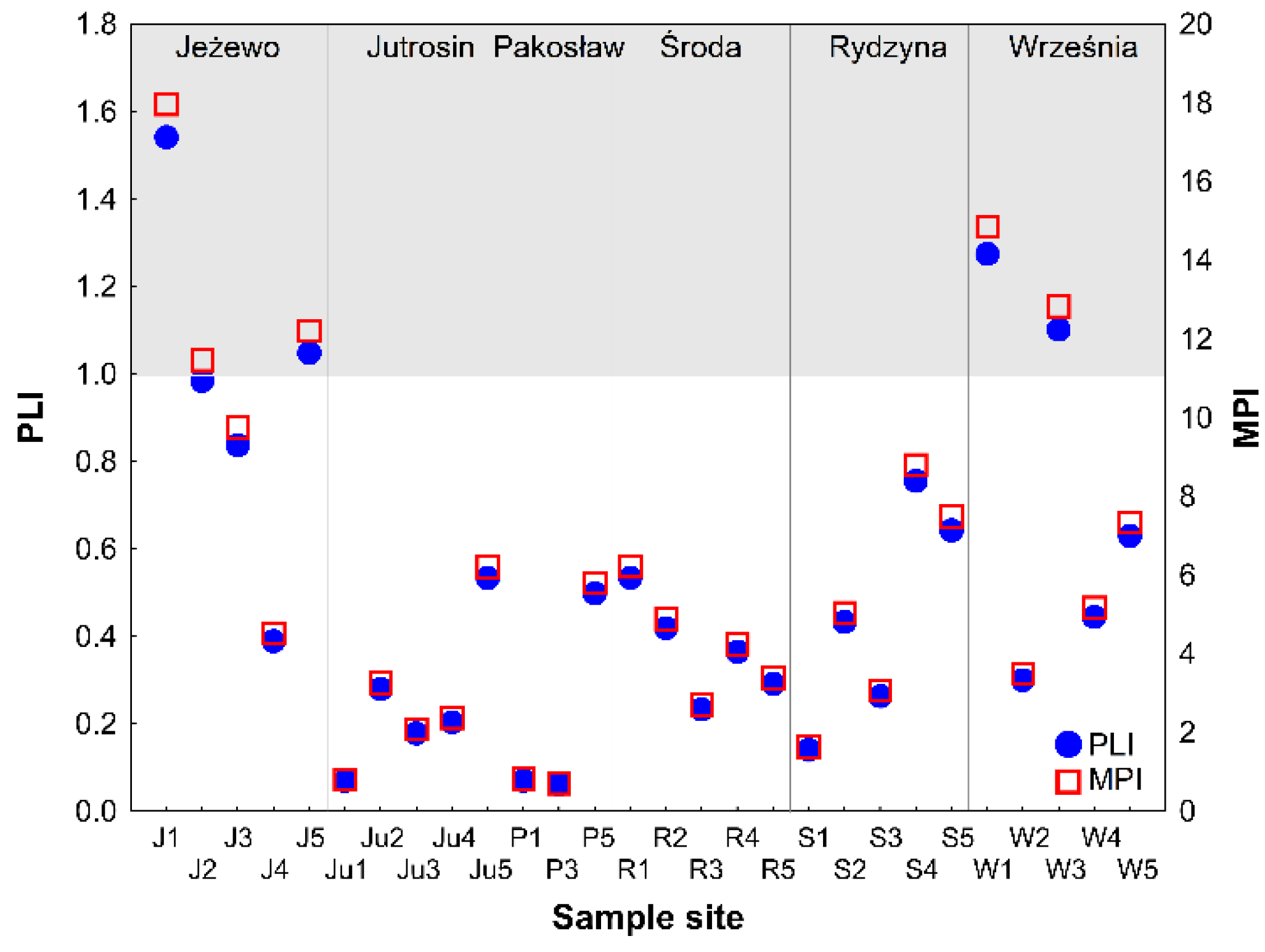
The enrichment factor (EF) was applied to assess the sources of HMs. The results of the EF calculations for Cd, Cr, Cu, Pb and Ni showed that the values generally did not exceed a value of 1 (Figure 2b). EF values ranging from 1 to 3 for Pb occurred once, for Cd and Cr twice, for Ni four times and for Cu nine times. In most cases, the values were less than 1.5, which may suggest that the HMs may come from natural weathering processes. In the case of Cr, at points S2 and W5 and for Cu at points S5 and W5, the EF values were higher than 1.5. However, an EF value higher than 1.5 indicates that HMs were delivered by other sources, such as point and non-point pollution [112,113]. The EF value of Zn was highest, and it ranged from 0.22 to 43.52. In fourteen sampling sites the EF values were higher than 3. Only in the Jutrosin reservoir were the EF values lower than 1. EF values for Zn higher than 10 were observed in the Jeżewo, Pakosław, Rydzyna, Środa and Września reservoirs, generally at sampling sites located at the inlet to the reservoir and at the dam. Two global indices of PLI and MPI were used to assess the bottom sediments’ contamination with HMs. PLI values ranged from 0.06 to 1.54. PLI values higher than 1 were noted four times at points J1, J5, W1 and W3 (Figure 3). These values may indicate the inflow of HMs from anthropogenic sources. The MPI index values ranged from 0.72 to 17.97. The highest MPI values occurred in the Jeżewo and Września reservoirs, on average 11.19 and 8.75 respectively. The lowest MPI values occurred in the Jutrosin and Pakosław reservoirs, 2.95 and 2.45 respectively (Figure 3). The highest values of the PLI and MPI indices were recorded at sampling sites located at the inlet to the reservoir and near the dam.
3.3. Ecological Risk Assessment
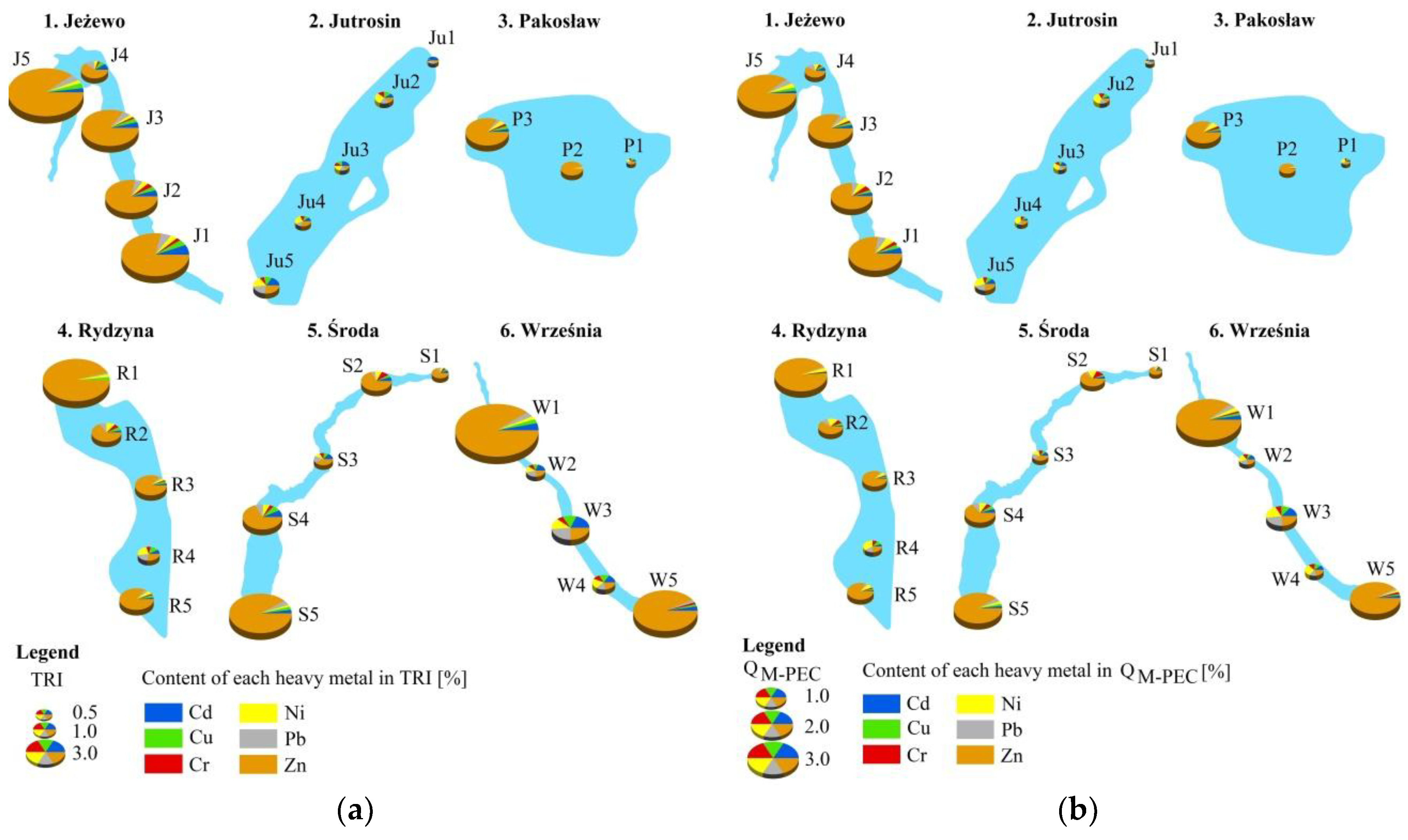
The toxic risk index was used to assess the toxic risk for HMs in bottom sediment samples. The values of the TRI index ranged from 0.17 to 13.56. In general, the TRI values were lower than 5 in 20 out of 28 sampling sites, which indicates a lack of ecological risk associated with HM concentrations in bottom sediments. Values lower than 5 occurred at all sampling sites located in Jutrosin reservoirs. TRI values ranging from 5 to 10 occurred six times (J1, J2, J3, R1, S5 and W5), which indicated low ecological risk. Only in sampling sites J5 and W1 were the TRI values higher than 10, which indicated moderate ecological risk. The highest contribution in the TRI index were Zn concentrations (Figure 4a), on average 59%. The average TRI value for the Jutrosin reservoir was the lowest at 0.64, while more than ten times higher values were found in the Jeżewo reservoir. The reservoirs according to TRI values can be arranged in ascending order Jutrosin < Pakosław < Środa < Rydzyna < Września < Jeżewo.
For the toxicity assessment of combined HMs, a consensus-based sediment quality guideline (SQG) was used. The Qm-PEC values ranged from 0.07 to 4.88. The average Qm-PEC values of the reservoirs ranked as follows: Jeżewo > Września > Rydzyna > Środa > Pakosław > Jutrosin. Qm-PEC values higher than 0.5 were noted up to seventeen times, which may indicate that HMs can be toxic to certain sediment-dwelling organisms [104]. Values higher than 0.5 occurred at all sampling sites located in the Jeżewo reservoir, four times in the Rydzyna reservoir and three times in the Środa and Września reservoirs (Figure 4b). The contribution of Zn was the highest in the Qm-PEC index of the analyzed sampling sites. However, at the sampling sites located in the Jutrosin reservoir and points W2, W3 and W4 (Września Reservoir), R4 (Rydzyna Reservoir) and S3 (Środa Reservoir), the percentages of HMs were at a similar level. It was observed that in the reservoirs, the greatest ecological risk associated with the pollution of HM deposits occurred at the inlet to the reservoir and near the dam.
3.4. Distribution and Source Identification
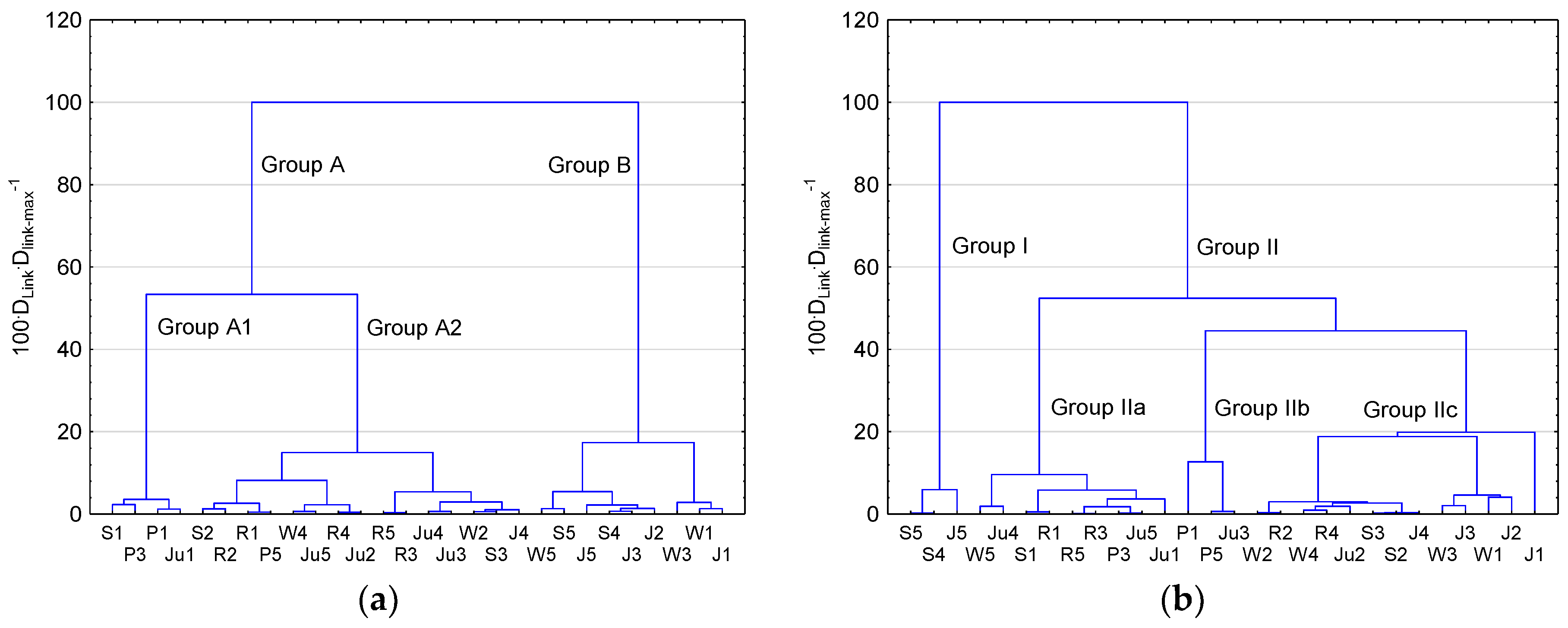
The CA analysis allowed the sampling sites to be divided into two groups, A and B, depending on the HM concentrations (Figure 5a). A total of 19 sampling sites were classified in group A and 9 in group B. The concentrations of all HMs in group A were lower than those observed in group B. In group B there are four measurement points located in the Jeżewo reservoir, three in the Września reservoir and two in the Środa reservoir. Group B was characterized by low variability of concentrations of individual HMs. Higher variability occurred in group A. Therefore, this group was divided into two subgroups: A1 and A2. Four sampling sites—S1, P1, Ju1 and P3—were classified in subgroup A1, in which the lowest concentrations of Cr, Ni, Cu and Pb were observed. However, in the case of Cd and Zn concentrations the differences between subgroups A1 and A2 were not statistically significant. Another division of the sampling sites into groups was obtained depending on the sediments’ bottom texture and TOM (Figure 5b). Samples were divided into two groups, I and II, which included 3 and 25 sampling sites, respectively. Sampling sites in group I were characterized by the highest content of TOM and silt fraction, on average 8.5% and 49.7%. At these sampling sites, the lowest sand fraction was observed, on average 47.0%. Within group II, 3 subgroups—IIa, IIb and IIc—were separated, into which 9, 3 and 13 sampling sites were classified respectively. In subgroup IIa there were sampling sites with the highest sand content (mean 92.9%) and the lowest content of silt and clay (average 6.7% and 0.4%). Also, the content of TOM was at the lowest level: 0.4%. Subgroup IIb was characterized by the highest content of clay (average 7.7%) and high content of sand (84.7%). In subgroup IIc the clay content was at a low level (on average 1.2%) and silt content at a high level (on average 21.8%). Dunn’s test showed that in groups I and II there are significant differences between sand, silt, clay and TOM content. Differences in all analyzed parameters were also present between subgroups IIa and IIc. However, between subgroups IIa and IIb there were only differences in the content of sand and clay and between subgroups IIb and IIc in the content of silt and clay. It was observed that the sample sites with the highest content of HMs (group B—Figure 5a) belonged to group I and subgroup IIc (Figure 5b). In these groups, high content of silt and TOM in group I was recorded.
3.5. Relationships between HM Concentrations and Sediment Texture and Organic Matter Content
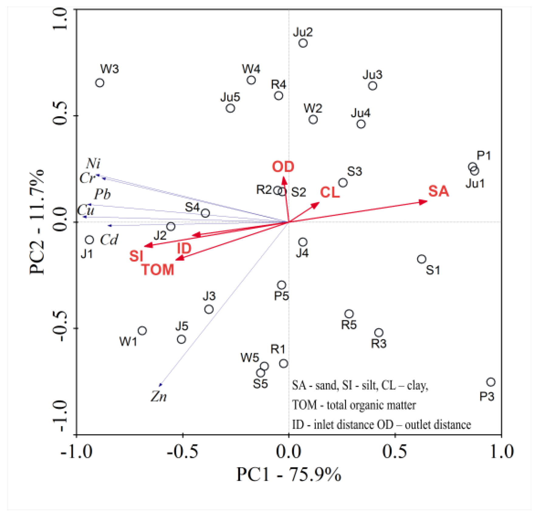
In the first stage, the aim of the PCA analysis was to identify factors that determine the concentration of HMs in the bottom sediments. The PCA analysis allowed two significant factors to be distinguished, PC1 and PC2, whose eigenvalues were higher than 1. The PC1 explains as much as 75.9% of the variance. The PC1 was strongly negatively correlated with Cd, Cr, Cu, Ni and Pb concentrations (Figure 6).
PC2, explaining about 11.7% of the variance, was strongly negatively correlated with Zn concentrations. The projection of sampling sites perpendicular to individual HM vectors or their extension beyond the origin of the coordinate system allows estimation of their content in bottom sediments. For example, the highest Zn values occur at sampling sites W1, J5, J1, S5, W5 and R1 and the lowest at sampling sites Ju3, Ju2, Ju1 and P1. The PC1 factor was moderately positively correlated with sand content and negatively with silt and TOM content. The angle created by the vectors of individual HMs informs about the relationship between them. The smaller the angle is, the stronger is the relationship; however, the angle value of 90° means no correlation. The analysis showed that the concentrations of HMs in bottom sediments are positively correlated with the silt content and negatively with the sand content (except Zn), while no correlations were observed with clay. In addition, the studies showed a positive correlation between Pb, Cu, Cd and Zn concentrations and TOM content. However, the relationship between individual HMs and silt was stronger than with TOM. A positive correlation was observed between the sampling site distance from the inlet to the reservoir (ID) and the silt and TOM content and a negative correlation with the sand content. This indicates grain size segregation in reservoirs. Thicker, sandy fractions are deposited at the inlet of the reservoirs, while the silt and TOM fractions are deposited near the dam.
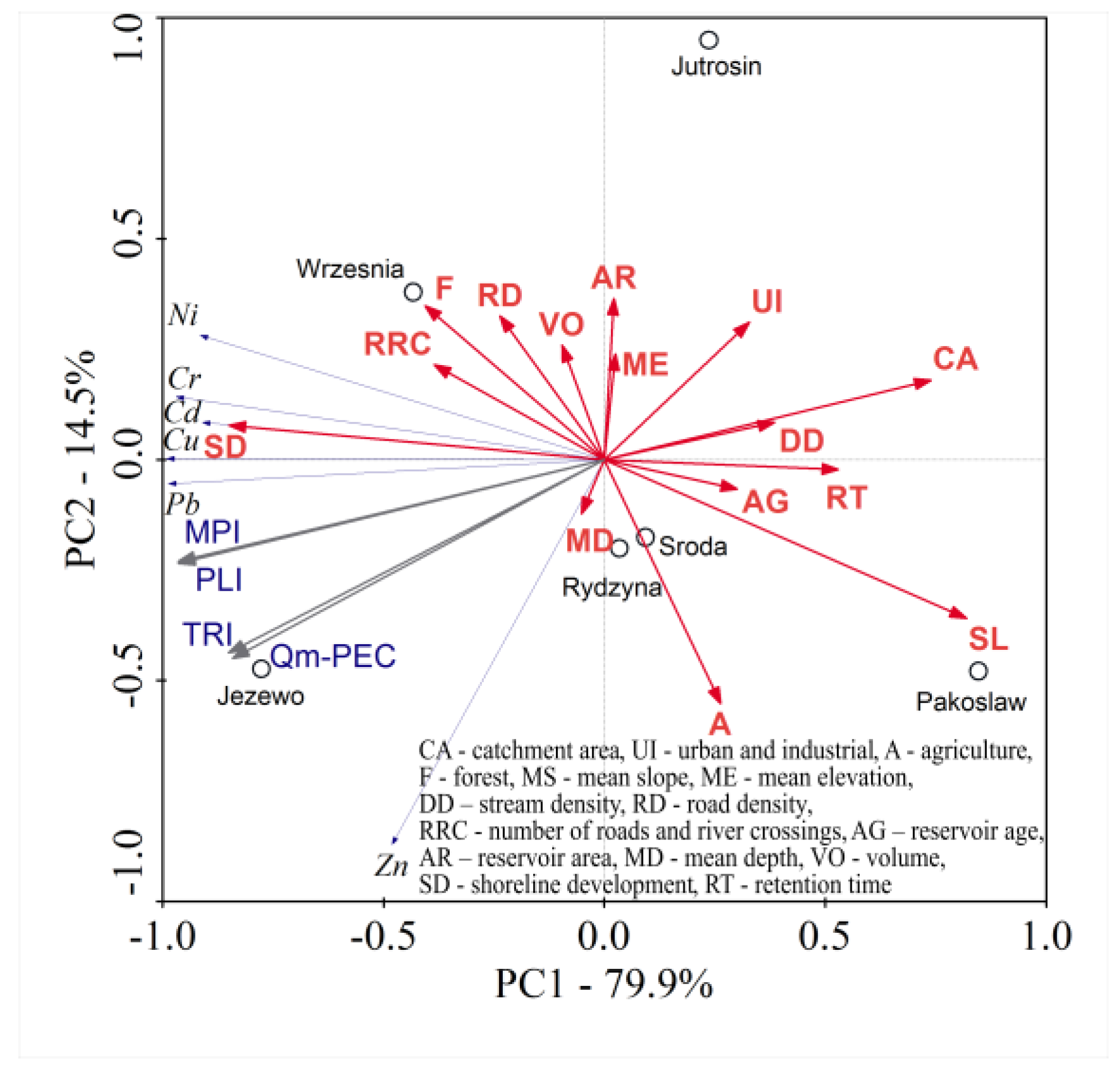
The second objective of the PCA was the identification of external factors that may affect the concentrations of HMs in reservoirs. The PCA analysis made it possible to distinguish two factors, PC1 and PC2, which explain 79.9 and 14.5% of variance respectively. The average concentrations of Cd, Cr, Cu, Ni and Pb were strongly negatively correlated with PC1, whereas Zn concentrations were strongly correlated with PC2 (Figure 7). Among the other factors that may have an impact on the content of HMs in bottom sediments, PC1 was strongly positively correlated with mean catchment slope and strongly negatively correlated with reservoir shoreline development. In addition, a positive correlation was observed with the catchment area and the water retention time in the reservoir. Only the share of agricultural areas was negatively correlated with PC2. The results indicate that HMs with the exception of Zn have the same source. Low concentrations in bottom sediments indicate that they originate from geogenic sources—weathering of rock material. The positive correlation with reservoir shoreline development indicates a possible impact of adjacent areas. The content of Ni in bottom sediments may additionally result from road traffic, which confirms the correlation with number of road and river crossings. The negative correlation of Cd, Cr, Cu, Pb and Ni with retention time indicates that in the reservoir with more frequent water exchange, HM concentrations are higher, which is related to the suspended sediment deposition, whereas the Zn in bottom sediments is correlated with agricultural land use. High concentrations of Zn in bottom sediments may result from the existence of anthropogenic sources and a potential supply with domestic wastewater. The data provided by the Central Statistical Office in Poland indicate that the number of people using the water supply network in the reservoir catchment varied from 93 to 98%. On the other hand, the number of people using the sewerage network varied from 36 to 65% for the Rydzyna and Września catchment respectively. The ratio of the length of the water supply to the length of the sewage system varied from 0.21 to 0.35. The above data indicate possible supply of Zn with domestic wastewater.
4. Discussion
The HM content in bottom sediments of retention reservoirs and relations between them result mainly from the impact of anthropogenic sources [14] as well as sediment texture and organic matter content [26]. Meteorological, hydrological and geological conditions of the catchment affect the content of sand, silt, clay and TOM in water. These factors influence the transport of HMs in the river-reservoir system. In the world, bottom sediments of retention reservoirs are characterized by relatively high variability of HM concentration. The analyzed reservoirs are located in agricultural catchment; therefore, HM concentrations in bottom sediments are at a lower level. Only Zn concentrations are at a higher level with respect to those noted by other authors in Polish reservoirs [25]. Probably Zn content may result from potential supply with domestic wastewater. The results presented in this paper confirmed the results obtained by Haziak et al. [114] which indicated that Zn values exceeding the geochemical background were associated with anthropogenic activities (run-off from farmland and domestic wastewater).
High values of the Igeo, EF, PLI and MPI indices at individual sampling sites of the reservoirs may suggest their origin of HMs from anthropogenic sources. High values at the inlet to the reservoir result from their inflow from point sources. Bing et al. [43] suggested that local anthropogenic activities increase contamination of specific HMs in the bottom sediments, especially of upper regions. Saleem et al. [55] observed relatively high content of HMs at sites which were adjacent to urban and semi-urban areas. The HMs may also come from the discharges of untreated urban/industrial wastes, agricultural runoffs and automobile emissions. High HM concentration near the dam is a consequence of changes in hydrological conditions in reservoirs during floods and high flow periods. HMs absorbed on silt and clay and TOM are transported and deposited near the dam. Also, Bing et al. [43] and Frémion et al. [17] reported relatively high values of HM concentrations close to the dam. Sojka et al. [25] noted that near the outlet pipe from the bottom sediments there can be discharged silt, clay and TOM, which are responsible for the transport of HM downstream from the reservoir.
The results have shown that concentrations of Cd, Cr, Cu, Ni, and Pb were strongly positively correlated with the silt and TOM contents in bottom sediments. However, the relationship with silt was at a higher level. Palma et al. [52] obtained slightly different results which showed stronger relationships between HMs and silt and clay content. However, the relationship between HMs and silt was stronger. Farhat and Aly [28] suggest that organic matter was more critical than grain size in controlling HM distribution in sediment. Different results were obtained by Frémion et al. [23], who found no relationships between trace elements and organic fraction.
The content in the bottom sediments of HMs involves the possibility of ecological risks. It was observed that the ecological risk in the reservoirs occurred at the inlet and near the dam, where the highest Qm-PEC and TRI values were obtained. Slightly different results were obtained by Bing et al. [43], who found that the potential ecological risk level increased towards the dam. Results obtained by Zhao et al. [50] suggested that the concentration and potential ecological risk of HMs in sediments near the dam were higher compared to the upstream sampling sites. The probable reason for the very high HM content at the reservoir’s inlet was the date of sampling during the very low flow period. The obtained values of Qm-PEC and TRI were the most strongly correlated with TOM. Our research confirmed the results obtained by Lin et al. [29] that the organic matter-bound fraction of heavy metal was a key mediator for ecological risk. Saleem et al. [55] demonstrated that organic matter may retain heavy elements in sediments and play an important role in bottom sediment quality assessment.
The present results showed that there is a strong correlation between Cd, Cr, Cu, Ni, and Pb. Suresh et al. [8] and Wang et al. [7] indicate that the HMs have common geochemical behaviors and originated from similar pollution sources when the correlation coefficient between them is higher. The absence of a correlation among the HMs suggests that the contents of these metals are not controlled by a single factor. Low concentrations of Cd, Cr, Cu, Ni, and Pb indicate their origin mainly from natural sources. In addition, during the research, the impact of the areas immediately adjacent to the reservoirs is marked; moreover, in the case of Ni the number of road and river crossings (RRC) plays an important role. Studies have shown that reservoirs with a shorter water retention time are more likely to supply HMs. In the case of Zn, it was shown that it may come from anthropogenic sources related to wastewater management in the reservoirs’ catchment.
5. Conclusions
The conducted analyses led us to draw the following conclusions:
- The content of HMs in bottom sediments is an individual feature of reservoirs.
- The PCA analysis and the values of Igeo, EF, MPI and PLI indices show that Cd, Cr, Cu, Ni and Pb in bottom sediments originate from geogenic sources – weathering of rock material. In contrast, Zn comes from anthropogenic sources.
- High variability of Zn concentrations between sampling sites and reservoirs confirms their origin from anthropogenic sources related to wastewater management.
- The PCA analysis indicates that the areas adjacent to reservoirs may have an impact on HM distribution, while the Ni concentration may additionally be affected by road traffic.
- In reservoirs with higher frequency of water exchange, higher HM concentrations were observed.
- The highest concentrations of HMs are observed at the inlet to the reservoir and near the dam, which causes the greatest ecological risk.
- The CA and PCA analysis show that the concentrations and spatial distribution of HMs depend on silt content. The Pb, Cu, Cd and Zn concentrations in reservoirs’ bottom sediments are associated with TOM content. However, the relation between individual HMs and silt was stronger than with TOM.
- Segregation of sediments along the reservoirs and the TOM content affect the concentrations and spatial distribution of HMs.
Author Contributions
Conceptualization—M.S. (Mariusz Sojka); methodology—M.S. (Mariusz Sojka) and J.J.; data collection—M.S. (Mariusz Sojka) and J.J.; chemical analyses—M.S. (Marcin Siepak); statistical analysis and interpretation—M.S. (Mariusz Sojka); writing—original draft preparation, M.S. (Mariusz Sojka); writing—review, M.S. (Mariusz Sojka); writing—editing, J.J.; visualization, M.S. (Mariusz Sojka) and J.J.; supervision—M.S. (Mariusz Sojka); project administration—M.S. (Mariusz Sojka).
Funding
This research was supported by financial means granted by the Ministry of Science and Higher Education; Research project No. 215862/E-336/SPUB/2017/1.
Conflicts of Interest
The authors declare no conflict of interest.
References
- Sojka, M.; Jaskuła, J.; Wicher-Dysarz, J.; Dysarz, T. The Impact of the Kowalskie Reservoir on the Hydrological Regime Alteration of the Główna River. J. Ecol. Eng. 2016, 17, 91–98. [Google Scholar] [CrossRef]
- Vukovic, D.; Vukovic, Z.; Stankovic, S. The impact of the Danube Iron Gate Dam on heavy metal storage and sediment flux within the reservoir. Catena 2014, 113, 18–23. [Google Scholar] [CrossRef]
- Dąbrowska, J.; Kaczmarek, H.; Markowska, J.; Tyszkowski, S.; Kempa, O.; Gałęza, M.; Kucharczak-Moryl, E.; Moryl, A. Shore zone in protection of water quality in agricultural landscape—The Mściwojów Reservoir, southwestern Poland. Environ. Monit. Assess. 2016, 188, 467. [Google Scholar] [CrossRef] [PubMed]
- Sedláček, J.; Bábek, O.; Nováková, T. Sedimentary record and anthropogenic pollution of a complex, multiple source fed dam reservoirs: An example from the Nové Mlýny reservoir, Czech Republic. Sci. Total Environ. 2017, 574, 1456–1471. [Google Scholar] [CrossRef] [PubMed]
- Bai, J.; Cui, B.; Chen, B.; Zhang, K.; Deng, W.; Gao, H.; Xiao, R. Spatial distribution and ecological risk assessment of heavy metals in surface sediments from a typical plateau lake wetland, China. Ecol. Modell. 2011, 222, 301–306. [Google Scholar] [CrossRef]
- Palma, P.; Ledo, L.; Alvarenga, P. Assessment of trace element pollution and its environmental risk to freshwater sediments influenced by anthropogenic contributions: The case study of Alqueva reservoir (Guadiana Basin). Catena 2015, 128, 174–184. [Google Scholar] [CrossRef] [Green Version]
- Wang, Y.; Yang, L.; Kong, L.; Liu, E.; Wang, L.; Zhu, J. Spatial distribution, ecological risk assessment and source identification for heavy metals in surface sediments from Dongping Lake, Shandong, East China. Catena 2015, 125, 200–205. [Google Scholar] [CrossRef]
- Suresh, G.; Sutharsan, P.; Ramasamy, V.; Venkatachalapathy, R. Assessment of spatial distribution and potential ecological risk of the heavy metals in relation to granulometric contents of Veeranam lake sediments, India. Ecotoxicol. Environ. Saf. 2012, 84, 117–124. [Google Scholar] [CrossRef]
- Barut, I.F.; Ergin, M.; Meriç, E.; Avşar, N.; Nazik, A.; Suner, F. Contribution of natural and anthropogenic effects in the Iznik Lake bottom sediment: Geochemical and microfauna assemblages evidence. Quat. Int. 2018, 486, 129–142. [Google Scholar] [CrossRef]
- Yazidi, A.; Saidi, S.; Mbarek, N.B.; Darragi, F. Contribution of GIS to evaluate surface water pollution by heavy metals: Case of Ichkeul Lake (Northern Tunisia). J. Afr. Earth Sci. 2017, 134, 166–173. [Google Scholar] [CrossRef]
- Lee, P.K.; Kang, M.J.; Yu, S.; Ko, K.S.; Ha, K.; Shin, S.C.; Park, J.H. Enrichment and geochemical mobility of heavy metals in bottom sediment of the Hoedong reservoir, Korea and their source apportionment. Chemosphere 2017, 184, 74–85. [Google Scholar] [CrossRef] [PubMed]
- Pavlović, P.; Mitrović, M.; Đorđević, D.; Sakan, S.; Slobodnik, J.; Liška, I.; Csanyi, B.; Jarić, S.; Kostić, O.; Pavlović, D.; et al. Assessment of the contamination of riparian soil and vegetation by trace metals—A Danube River case study. Sci. Total Environ. 2016, 540, 396–409. [Google Scholar] [CrossRef] [PubMed]
- Wang, L.F.; Yang, L.Y.; Kong, L.H.; Li, S.; Zhu, J.R.; Wang, Y.Q. Spatial distribution, source identification and pollution assessment of metal content in the surface sediments of Nansi Lake, China. J. Geochem. Explor. 2014, 140, 87–95. [Google Scholar] [CrossRef]
- Wang, X.; Zhang, L.; Zhao, Z.; Cai, Y. Heavy metal pollution in reservoirs in the hilly area of southern China: Distribution, source apportionment and health risk assessment. Sci. Total Environ. 2018, 634, 158–169. [Google Scholar] [CrossRef] [PubMed]
- Noronha-D’Mello, C.A.; Nayak, G.N. Assessment of metal enrichment and their bioavailability in sediment and bioaccumulation by mangrove plant pneumatophores in a tropical (Zuari) estuary, west coast of India. Mar. Pollut. Bull. 2016, 110, 221–230. [Google Scholar] [CrossRef]
- Sojka, M.; Siepak, M.; Jaskuła, J.; Wicher-Dysarz, J. Heavy Metal Transport in a River-Reservoir System: A Case Study from Central Poland. Pol. J. Environ. Stud. 2018, 27, 1725–1734. [Google Scholar] [CrossRef]
- Frémion, F.; Courtin-Nomade, A.; Bordas, F.; Lenain, J.F.; Jugé, P.; Kestens, T.; Mourier, B. Impact of sediments resuspension on metal solubilization and water quality during recurrent reservoir sluicing management. Sci. Total Environ. 2016, 562, 201–215. [Google Scholar] [CrossRef]
- Wang, C.Y.; Wang, X.L. Spatial distribution of dissolved Pb, Hg, Cd, Cu and as in the Bohai sea. J. Environ. Sci. (China) 2007, 19, 1061–1066. [Google Scholar] [CrossRef]
- Wilson, D.C. Potential urban runoff impacts and contaminant distributions in shoreline and reservoir environments of Lake Havasu, southwestern United States. Sci. Total Environ. 2018, 621, 95–107. [Google Scholar] [CrossRef]
- Morris, G.L.; Fan, J. Reservoir Sedimentation Handbook: Design and Management of Dams, Reservoirs, and Watersheds for Sustainable Use; McGraw-Hill Publishing Co.: New York, NY, USA, 1998; ISBN 978-0070433021. [Google Scholar]
- Wang, Y.; Hu, J.; Xiong, K.; Huang, X.; Duan, S. Distribution of heavy metals in core sediments from Baihua Lake. Procedia Environ. Sci. 2012, 16, 51–58. [Google Scholar] [CrossRef]
- Yujun, Y.; Zhaoyin, W.; Zhang, K.; Guoan, Y.U.; Xuehua, D. Sediment pollution and its effect on fish through food chain in the Yangtze River. Int. J. Sediment Res. 2008, 23, 338–347. [Google Scholar] [CrossRef]
- Frémion, F.; Bordas, F.; Mourier, B.; Lenain, J.F.; Kestens, T.; Courtin-Nomade, A. Influence of dams on sediment continuity: A study case of a natural metallic contamination. Sci. Total Environ. 2016, 547, 282–294. [Google Scholar] [CrossRef] [PubMed]
- Redwan, M.; Elhaddad, E. Heavy metals seasonal variability and distribution in Lake Qaroun sediments, El-Fayoum, Egypt. J. Afr. Earth Sci. 2017, 134, 48–55. [Google Scholar] [CrossRef]
- Sojka, M.; Siepak, M.; Gnojska, E. Assessment of heavy metal concentration in bottom sediments of Stare Miasto pre-dam reservoir on the Powa river. Annu. Set Environ. Prot. 2013, 15, 1916–1928. [Google Scholar]
- Lin, Q.; Liu, E.; Zhang, E.; Li, K.; Shen, J. Spatial distribution, contamination and ecological risk assessment of heavy metals in surface sediments of Erhai Lake, a large eutrophic plateau lake in southwest China. Catena 2016, 145, 193–203. [Google Scholar] [CrossRef]
- Frankowski, M.; Sojka, M.; Zioła-Frankowska, A.; Siepak, M.; Murat-Błażejewska, S. Distribution of heavy metals in the Mała Wełna River system (western Poland). Oceanol. Hydrobiol. Stud. 2009, 38, 51–61. [Google Scholar] [CrossRef]
- Farhat, H.I.; Aly, W. Effect of site on sedimentological characteristics and metal pollution in two semi-enclosed embayments of great freshwater reservoir: Lake Nasser, Egypt. J. Afr. Earth Sci. 2018, 141, 194–206. [Google Scholar] [CrossRef]
- Lin, J.; Zhang, S.; Liu, D.; Yu, Z.; Zhang, L.; Cui, J.; Xie, K.; Li, T.; Fu, C. Mobility and potential risk of sediment-associated heavy metal fractions under continuous drought-rewetting cycles. Sci. Total Environ. 2018, 625, 79–86. [Google Scholar] [CrossRef]
- Martínez-Santos, M.; Probst, A.; García-García, J.; Ruiz-Romera, E. Influence of anthropogenic inputs and a high-magnitude flood event on metal contamination pattern in surface bottom sediments from the Deba River urban catchment. Sci. Total Environ. 2015, 514, 10–25. [Google Scholar] [CrossRef] [Green Version]
- Zhang, Z.; Juying, L.; Mamat, Z.; QingFu, Y. Sources identification and pollution evaluation of heavy metals in the surface sediments of Bortala River, Northwest China. Ecotoxicol. Environ. Saf. 2016, 126, 94–101. [Google Scholar] [CrossRef]
- Dong, A.; Zhai, S.; Zabel, M.; Yu, Z.; Zhang, H.; Liu, F. Heavy metals in Changjiang estuarine and offshore sediments: Responding to human activities. Acta Oceanol. Sin. 2012, 31, 88–101. [Google Scholar] [CrossRef]
- Dhanakumar, S.; Murthy, K.R.; Solaraj, G.; Mohanraj, R. Heavy-metal fractionation in surface sediments of the Cauvery River estuarine region, southeastern coast of India. Arch. Environ. Contam. Toxicol. 2013, 65, 14–23. [Google Scholar] [CrossRef] [PubMed]
- Zhang, C.; Yu, Z.G.; Zeng, G.M.; Jiang, M.; Yang, Z.Z.; Cui, F.; Zhu, M.; Shen, L.; Hu, L. Effects of sediment geochemical properties on heavy metal bioavailability. Environ. Int. 2014, 73, 270–281. [Google Scholar] [CrossRef] [PubMed]
- Graham, M.C.; Gavin, K.G.; Kirika, A.; Farmer, J.G. Processes controlling manganese distributions and associations in organic-rich freshwater aquatic systems: The example of Loch Bradan, Scotland. Sci. Total Environ. 2012, 424, 239–250. [Google Scholar] [CrossRef] [PubMed]
- Zhong, A.P.; Guo, S.H.; Li, F.M.; Gang, L.I.; Jiang, K.X. Impact of anions on the heavy metals release from marine sediments. J. Environ. Sci. 2006, 18, 1216–1220. [Google Scholar] [CrossRef]
- Du Laing, G.; De Vos, R.; Vandecasteele, B.; Lesage, E.; Tack, F.M.; Verloo, M.G. Effect of salinity on heavy metal mobility and availability in intertidal sediments of the Scheldt estuary. Estuar. Coast. Shelf Sci. 2008, 77, 589–602. [Google Scholar] [CrossRef]
- Dhanakumar, S.; Solaraj, G.; Mohanraj, R. Heavy metal partitioning in sediments and bioaccumulation in commercial fish species of three major reservoirs of river Cauvery delta region, India. Ecotoxicol. Environ. Saf. 2015, 113, 145–151. [Google Scholar] [CrossRef]
- Zhu, L.; Liu, J.; Xu, S.; Xie, Z. Deposition behavior, risk assessment and source identification of heavy metals in reservoir sediments of Northeast China. Ecotoxicol. Environ. Saf. 2017, 142, 454–463. [Google Scholar] [CrossRef]
- Yi, Y.; Yang, Z.; Zhang, S. Ecological risk assessment of heavy metals in sediment and human health risk assessment of heavy metals in fishes in the middle and lower reaches of the Yangtze River basin. Environ. Pollut. 2011, 159, 2575–2585. [Google Scholar] [CrossRef]
- Zhuang, W.; Liu, Y.; Chen, Q.; Wang, Q.; Zhou, F. A new index for assessing heavy metal contamination in sediments of the Beijing-Hangzhou Grand Canal (Zaozhuang Segment): A case study. Ecol. Indic. 2016, 69, 252–260. [Google Scholar] [CrossRef] [Green Version]
- Birch, G.F.; Apostolatos, C. Use of sedimentary metals to predict metal concentrations in black mussel (Mytilus galloprovincialis) tissue and risk to human health (Sydney estuary, Australia). Environ. Sci. Pollut. Res. Int. 2013, 20, 5481–5491. [Google Scholar] [CrossRef] [PubMed]
- Bing, H.; Wu, Y.; Zhou, J.; Sun, H.; Wang, X.; Zhu, H. Spatial variation of heavy metal contamination in the riparian sediments after two-year flow regulation in the Three Gorges Reservoir, China. Sci. Total Environ. 2019, 649, 1004–1016. [Google Scholar] [CrossRef] [PubMed]
- Song, J.; Duan, X.; Han, X.; Li, Y.; Li, Y.; He, D. The accumulation and redistribution of heavy metals in the water-level fluctuation zone of the Nuozhadu Reservoir, Upper Mekong. Catena 2019, 172, 335–344. [Google Scholar] [CrossRef]
- Fathollahzadeh, H.; Kaczala, F.; Bhatnagar, A.; Hogland, W. Significance of environmental dredging on metal mobility from contaminated sediments in the Oskarshamn Harbor, Sweden. Chemosphere 2015, 119, 445–451. [Google Scholar] [CrossRef] [PubMed]
- Wang, C.; Liu, S.; Zhao, Q.; Deng, L.; Dong, S. Spatial variation and contamination assessment of heavy metals in sediments in the Manwan Reservoir, Lancang River. Ecotoxicol. Environ. Saf. 2012, 82, 32–39. [Google Scholar] [CrossRef]
- Peraza-Castro, M.; Sauvage, S.; Sánchez-Pérez, J.M.; Ruiz-Romera, E. Effect of flood events on transport of suspended sediments, organic matter and particulate metals in a forest watershed in the Basque Country (Northern Spain). Sci. Total Environ. 2016, 569, 784–797. [Google Scholar] [CrossRef]
- Hahn, J.; Opp, C.; Evgrafova, A.; Groll, M.; Zitzer, N.; Laufenberg, G. Impacts of dam draining on the mobility of heavy metals and arsenic in water and basin bottom sediments of three studied dams in Germany. Sci. Total Environ. 2018, 640, 1072–1081. [Google Scholar] [CrossRef]
- Fu, K.D.; Su, B.; He, D.M.; Lu, X.X.; Song, J.Y.; Huang, J.C. Pollution assessment of heavy metals along the Mekong River and dam effects. J. Geogr. Sci. 2012, 22, 874–884. [Google Scholar] [CrossRef]
- Zhao, Q.; Liu, S.; Deng, L.; Dong, S.; Wang, C. Longitudinal distribution of heavy metals in sediments of a canyon reservoir in Southwest China due to dam construction. Environ. Monit. Assess. 2013, 185, 6101–6110. [Google Scholar] [CrossRef]
- Dai, Z.; Liu, J.T. Impacts of large dams on downstream fluvial sedimentation: An example of the Three Gorges Dam (TGD) on the Changjiang (Yangtze River). J. Hydrol. 2013, 480, 10–18. [Google Scholar] [CrossRef]
- Palma, P.; Ledo, L.; Soares, S.; Barbosa, I.R.; Alvarenga, P. Spatial and temporal variability of the water and sediments quality in the Alqueva reservoir (Guadiana Basin; southern Portugal). Sci. Total Environ. 2014, 470, 780–790. [Google Scholar] [CrossRef] [PubMed]
- Li, F.; Zhang, J.; Liu, C.; Xiao, M.; Wu, Z. Distribution, bioavailability and probabilistic integrated ecological risk assessment of heavy metals in sediments from Honghu Lake, China. Process. Saf. Environ. Prot. 2018, 116, 169–179. [Google Scholar] [CrossRef]
- Zhang, C.; Shan, B.; Zhao, Y.; Song, Z.; Tang, W. Spatial distribution, fractionation, toxicity and risk assessment of surface sediments from the Baiyangdian Lake in northern China. Ecol. Indic. 2018, 90, 633–642. [Google Scholar] [CrossRef]
- Saleem, M.; Iqbal, J.; Akhter, G.; Shah, M.H. Fractionation, bioavailability, contamination and environmental risk of heavy metals in the sediments from a freshwater reservoir, Pakistan. J. Geochem. Explor. 2018, 184, 199–208. [Google Scholar] [CrossRef]
- Dummee, V.; Kruatrachue, M.; Trinachartvanit, W.; Tanhan, P.; Pokethitiyook, P.; Damrongphol, P. Bioaccumulation of heavy metals in water, sediments, aquatic plant and histopathological effects on the golden apple snail in Beung Boraphet reservoir, Thailand. Ecotoxicol. Environ. Saf. 2012, 86, 204–212. [Google Scholar] [CrossRef] [PubMed]
- Ji, H.; Ding, H.; Tang, L.; Li, C.; Gao, Y.; Briki, M. Chemical composition and transportation characteristic of trace metals in suspended particulate matter collected upstream of a metropolitan drinking water source, Beijing. J. Geochem. Explor. 2016, 169, 123–136. [Google Scholar] [CrossRef]
- Bing, H.; Zhou, J.; Wu, Y.; Wang, X.; Sun, H.; Li, R. Current state, sources, and potential risk of heavy metals in sediments of Three Gorges Reservoir, China. Environ. Pollut. 2016, 214, 485–496. [Google Scholar] [CrossRef]
- Hanif, N.; Eqani, S.A.M.A.S.; Ali, S.M.; Cincinelli, A.; Ali, N.; Katsoyiannis, I.A.; Tanveer, Z.I.; Bokhari, H. Geo-accumulation and enrichment of trace metals in sediments and their associated risks in the Chenab River, Pakistan. J. Geochem. Explor. 2016, 165, 62–70. [Google Scholar] [CrossRef]
- El-Amier, Y.A.; Elnaggar, A.; El-Alfy, M.A. Evaluation and mapping spatial distribution of bottom sediment heavy metal contamination in Burullus Lake, Egypt. Egypt. J. Basic Appl. Sci. 2017, 4, 55–66. [Google Scholar] [CrossRef]
- Ali, M.M.; Ali, M.L.; Islam, M.S.; Rahman, M.Z. Preliminary assessment of heavy metals in water and sediment of Karnaphuli River, Bangladesh. Environ. Nanotechnol. Monit. Manag. 2016, 5, 27–35. [Google Scholar] [CrossRef]
- Audry, S.; Schäfer, J.; Blanc, G.; Jouanneau, J.M. Fifty-year sedimentary record of heavy metal pollution (Cd, Zn, Cu, Pb) in the Lot River reservoirs (France). Environ. Pollut. 2004, 132, 413–426. [Google Scholar] [CrossRef] [PubMed]
- Bian, B.; Zhou, Y.; Fang, B.B. Distribution of heavy metals and benthic macroinvertebrates: Impacts from typical inflow river sediments in the Taihu Basin, China. Ecol. Indic. 2016, 69, 348–359. [Google Scholar] [CrossRef]
- El-Sayed, S.A.; Moussa, E.M.M.; El-Sabagh, M.E.I. Evaluation of heavy metal content in Qaroun Lake, El-Fayoum, Egypt. Part I: Bottom sediments. J. Radiat. Res. Appl. Sci. 2015, 8, 276–285. [Google Scholar] [CrossRef]
- Gu, J.; Salem, A.; Chen, Z. Lagoons of the Nile delta, Egypt, heavy metal sink: With a special reference to the Yangtze estuary of China. Estuar. Coast. Shelf Sc. 2013, 117, 282–292. [Google Scholar] [CrossRef]
- Mohamaden, M.I.; Khalil, M.K.; Draz, S.E.; Hamoda, A.Z. Ecological risk assessment and spatial distribution of some heavy metals in surface sediments of New Valley, Western Desert, Egypt. Egypt. J. Aquat. Res. 2017, 43, 31–43. [Google Scholar] [CrossRef]
- Zahra, A.; Hashmi, M.Z.; Malik, R.N.; Ahmed, Z. Enrichment and geo-accumulation of heavy metals and risk assessment of sediments of the Kurang Nallah—Feeding tributary of the Rawal Lake Reservoir, Pakistan. Sci. Total Environ. 2014, 470, 925–933. [Google Scholar] [CrossRef] [PubMed]
- Zhang, W.; Feng, H.; Chang, J.; Qu, J.; Xie, H.; Yu, L. Heavy metal contamination in surface sediments of Yangtze River intertidal zone: An assessment from different indexes. Environ. Pollut. 2009, 157, 1533–1543. [Google Scholar] [CrossRef]
- Lario, J.; Alonso-Azcárate, J.; Spencer, C.; Zazo, C.; Goy, J.L.; Cabero, A.; Dabrio, C.J.; Borja, F.; Borja, C.; Civis, J.; et al. Evolution of the pollution in the Piedras river natural site (Gulf of cadiz, southern Spain) during the holocene. Environ. Earth Sci. 2016, 75, 481. [Google Scholar] [CrossRef]
- Wang, G.; Yinglan, A.; Jiang, H.; Fu, Q.; Zheng, B. Modeling the source contribution of heavy metals in surficial sediment and analysis of their historical changes in the vertical sediments of a drinking water reservoir. J. Hydrol. 2015, 520, 37–51. [Google Scholar] [CrossRef]
- Li, F.; Huang, J.; Zeng, G.; Yuan, X.; Li, X.; Liang, J.; Wang, X.; Tang, X.; Bai, B. Spatial risk assessment and sources identification of heavy metals in surface sediments from the Dongting Lake, Middle China. J. Geochem. Explor. 2013, 132, 75–83. [Google Scholar] [CrossRef]
- Wang, L.; Dai, L.; Li, L.; Liang, T. Multivariable cokriging prediction and source analysis of potentially toxic elements (Cr, Cu, Cd, Pb, and Zn) in surface sediments from Dongting Lake, China. Ecol. Indic. 2018, 94, 312–319. [Google Scholar] [CrossRef]
- Siepak, M.; Sojka, M. Application of multivariate statistical approach to identify trace elements sources in surface waters: A case study of Kowalskie and Stare Miasto reservoirs, Poland. Environ. Monit. Assess. 2017, 189, 364. [Google Scholar] [CrossRef] [PubMed]
- Sojka, M.; Siepak, M.; Zioła, A.; Frankowski, M.; Murat-Błażejewska, S. Application of multivariate statistical techniques to evaluation of water quality in the Mała Wełna River (Western Poland). Environ. Monit. Assess. 2008, 147, 159–170. [Google Scholar] [CrossRef] [PubMed]
- Sojka, M.; Siepak, M.; Pietrewicz, K. Concentration of Rare Earth Elements in surface water and bottom sediments in Lake Wadąg, Poland. J. Elem. 2019, 24, 125–140. [Google Scholar] [CrossRef]
- Przybyła, C.; Kozdrój, P.; Sojka, M. Application of Multivariate Statistical Methods in Water Quality Assessment of River-reservoirs Systems (on the Example of Jutrosin and Pakosław Reservoirs, Orla Basin). Annu. Set Environ. Prot. 2015, 17, 1125–1141. [Google Scholar]
- Ye, C.; Li, S.; Zhang, Y.; Zhang, Q. Assessing soil heavy metal pollution in the water-level-fluctuation zone of the Three Gorges Reservoir, China. J. Hazard Mater. 2011, 191, 366–372. [Google Scholar] [CrossRef] [PubMed]
- Wu, Q.; Qi, J.; Xia, X. Long-term variations in sediment heavy metals of a reservoir with changing trophic states: Implications for the impact of climate change. Sci. Total Environ. 2017, 609, 242–250. [Google Scholar] [CrossRef] [PubMed]
- Sojka, M. Assessment of biogenic compounds eluted from the catchment of Dembina river. Annu. Set Environ. Prot. 2009, 11, 1225–1234. [Google Scholar]
- Sojka, M.; Murat-Błażejewska, S. Physico-chemical and hydromorphological state of a small lowland river. Annu. Set Environ. Prot. 2009, 11, 727–737. [Google Scholar]
- Sojka, M.; Korytowski, M.; Jaskuła, J.; Waligórski, B. Assessment of vulnerability to degradation of the Przebędowo reservoir. J. Ecol. Eng. 2017, 18, 118–125. [Google Scholar] [CrossRef] [Green Version]
- Sojka, M.; Jaskuła, J.; Wicher-Dysarz, J.; Dysarz, T. Analysis of selected reservoirs functioning in the Wielkopolska region. Acta Sci. Pol. Formatio Circumiectus 2017, 16, 205–215. [Google Scholar] [CrossRef]
- Jaskuła, J.; Sojka, M.; Wicher-Dysarz, J. Analysis of the vegetation process in a two-stage reservoir on the basis of satellite imagery - a case study: Radzyny reservoir on the Sama river. Annu. Set Environ. Prot. 2018, 20, 203–220. [Google Scholar]
- Sojka, M.; Jaskuła, J.; Wróżyński, R.; Waligórski, B. Application of Sentinel-2 satellite imagery to assessment of spatio-temporal changes in the reservoir overgrowth process—A case study: Przebędowo, West Poland. Carpath. J. Earth Environ. 2019, 14, 39–50. [Google Scholar] [CrossRef]
- Baran, A.; Tarnawski, M.; Koniarz, T. Spatial distribution of trace elements and ecotoxicity of bottom sediments in Rybnik reservoir, Silesian-Poland. Environ. Sci. Pollut. Res. Int. 2016, 23, 17255–17268. [Google Scholar] [CrossRef] [PubMed] [Green Version]
- Wiatkowski, M. Problems of water management in the reservoir Młyny located on the Julianpolka river. Acta Sci. Pol. Formatio Circumiectus 2015, 14, 191–203. [Google Scholar] [CrossRef]
- Kasperek, R.; Wiatkowski, M. Bottom studies of Mściwojów reservoir. Sci. Rev. Eng. Environ. Sci. 2008, 17, 194–201. [Google Scholar]
- Smal, H.; Ligęza, S.; Wójcikowska-Kapusta, A.; Baran, S.; Urban, D.; Obroślak, R.; Pawłowski, A. Spatial distribution and risk assessment of heavy metals in bottom sediments of two small dam reservoirs (south-east Poland). Arch. Environ. Prot. 2015, 41, 67–80. [Google Scholar] [CrossRef] [Green Version]
- Cymes, I.; Glińska-Lewczuk, K.; Szymczyk, S.; Sidoruk, M.; Potasznik, A. Distribution and potential risk assessment of heavy metals and arsenic in sediments of a dam reservoir: A case study of the Łoje Retention Reservoir, NE Poland. J. Elem. 2017, 22, 843–856. [Google Scholar] [CrossRef]
- Łabędzki, L. Estimation of local drought frequency in central Poland using the standardized precipitation index SPI. Irrig. Drainage 2007, 56, 67–77. [Google Scholar] [CrossRef]
- Ostrowska, A.; Gawliński, S.; Szczubiałka, Z. Methods of Analysis and Assessment of Soil and Plant Properties; Environmental Protection Institute: Warsaw, Poland, 1991. [Google Scholar]
- Müller, G. Schwermetalle in den Sedimenten des Rheins—Veränderungen seit 1971. Umschau 1979, 79, 778–783. [Google Scholar]
- Benhaddya, M.L.; Hadjel, M. Spatial distribution and contamination assessment of heavy metals in surface soils of Hassi Messaoud, Algeria. Environ. Earth Sci. 2014, 71, 1473–1486. [Google Scholar] [CrossRef]
- Deely, J.M.; Fergusson, J.E. Heavy metal and organic matter concentrations and distributions in dated sediments of a small estuary adjacent to a small urban area. Sci. Total Environ. 1994, 153, 97–111. [Google Scholar] [CrossRef]
- Ergin, M.; Saydam, C.; Baştürk, Ö.; Erdem, E.; Yörük, R. Heavy metal concentrations in surface sediments from the two coastal inlets (Golden Horn Estuary and Izmit Bay) of the northeastern Sea of Marmara. Chem. Geol. 1991, 91, 269–285. [Google Scholar] [CrossRef]
- Aiman, U.; Mahmood, A.; Waheed, S.; Malik, R.N. Enrichment, geo-accumulation and risk surveillance of toxic metals for different environmental compartments from Mehmood Booti dumping site, Lahore city, Pakistan. Chemosphere 2016, 144, 2229–2237. [Google Scholar] [CrossRef]
- Islam, M.S.; Ahmed, M.K.; Raknuzzaman, M.; Habibullah-Al-Mamun, M.; Islam, M.K. Heavy metal pollution in surface water and sediment: A preliminary assessment of an urban river in a developing country. Ecol. Indic. 2015, 48, 282–291. [Google Scholar] [CrossRef]
- Al Rashdi, S.; Arabi, A.A.; Howari, F.M.; Siad, A. Distribution of heavy metals in the coastal area of Abu Dhabi in the United Arab Emirates. Mar. Pollut. Bull. 2015, 97, 494–498. [Google Scholar] [CrossRef] [PubMed]
- Sakan, S.M.; Đorđević, D.S.; Manojlović, D.D.; Predrag, P.S. Assessment of heavy metal pollutants accumulation in the Tisza river sediments. J. Environ. Manag. 2009, 90, 3382–3390. [Google Scholar] [CrossRef] [PubMed]
- Tomlinson, D.L.; Wilson, J.G.; Harris, C.R.; Jeffrey, D.W. Problems in the assessment of heavy-metal levels in estuaries and the formation of a pollution index. Helgol. Mar. Res. 1980, 33, 566–575. [Google Scholar] [CrossRef] [Green Version]
- Harikumar, P.S.; Nasir, U.P.; Rahman, M.M. Distribution of heavy metals in the core sediments of a tropical wetland system. Int. J. Environ. Sci. Technol. 2009, 6, 225–232. [Google Scholar] [CrossRef] [Green Version]
- Usero, J.; Morillo, J.; Gracia, I. Heavy metal concentrations in molluscs from the Atlantic coast of southern Spain. Chemosphere 2005, 59, 1175–1181. [Google Scholar] [CrossRef]
- Bojakowska, I.; Sokołowska, G. Geochemiczne klasy czystości osadów wodnych. Przegląd Geologiczny 1998, 46, 49–54. [Google Scholar]
- MacDonald, D.D.; Ingersoll, C.G.; Berger, T.A. Development and evaluation of consensus-based sediment quality guidelines for freshwater ecosystems. Arch. Environ. Contam. Toxicol. 2000, 39, 20–31. [Google Scholar] [CrossRef] [PubMed]
- Fu, J.; Zhao, C.; Luo, Y.; Liu, C.; Kyzas, G.Z.; Luo, Y.; Zhu, H. Heavy metals in surface sediments of the Jialu River. China: Their relations to environmental factors. J. Hazard Mater. 2014, 270, 102–109. [Google Scholar] [CrossRef] [PubMed]
- Lecce, S.A.; Pavlowsky, R.T. Floodplain storage of sediment contaminated by mercury and copper from historic gold mining at Gold Hill. North Carolina. USA. Geomorphology 2014, 206, 122–132. [Google Scholar] [CrossRef]
- Zhang, G.; Bai, J.; Zhao, Q.; Lu, Q.; Jia, J.; Wen, X. Heavy metals in wetland soils along a wetland-forming chronosequence in the Yellow River Delta of China: Levels, sources and toxic risks. Ecol. Indic. 2016, 69, 331–339. [Google Scholar] [CrossRef]
- Long, E.R.; MacDonald, D.D. Recommended uses of empirically derived. sediment quality guidelines for marine and estuarine ecosystems. Hum. Ecol. Risk Assess. 1998, 4, 1019–1039. [Google Scholar] [CrossRef]
- Ptak, M.; Sojka, M.; Choiński, A.; Nowak, B. Effect of Environmental Conditions and Morphometric Parameters on Surface Water Temperature in Polish Lakes. Water 2018, 10, 580. [Google Scholar] [CrossRef]
- Glińska-Lewczuk, K.; Burandt, P.; Kujawa, R.; Kobus, S.; Obolewski, K.; Dunalska, J.; Grabowska, M.; Lew, S.; Chormański, J. Environmental factors structuring fish communities in floodplain lakes of the undisturbed system of the Biebrza River. Water 2016, 8, 146. [Google Scholar] [CrossRef]
- Liu, C.W.; Lin, K.H.; Kuo, Y.M. Application of factor analysis in the assessment of groundwater quality in blackfoot disease in Taiwan. Sci. Total Environ. 2003, 313, 77–89. [Google Scholar] [CrossRef]
- Yongming, H.; Peixuan, D.; Junji, C.; Posmentier, E.S. Multivariate analysis of heavy metal contamination in urban dusts of Xi’an, Central China. Sci. Total Environ. 2006, 355, 176–186. [Google Scholar] [CrossRef]
- Zhang, J.; Liu, C.L. Riverine composition and estuarine geochemistry of particulate metals in China—Weathering features, anthropogenic impact and chemical fluxes. Estuar. Coast. Shelf Sci. 2002, 54, 1051–1070. [Google Scholar] [CrossRef]
- Haziak, T.; Czaplicka-Kotas, A.; Ślusarczyk, Z.; Szalińska, E. Spatial changes of zinc concentrations in the Czorsztyn reservoir sediments. Eng. Prot. Environ. 2013, 16, 57–68. [Google Scholar]
Figure 1.
Study site location.

Figure 2.
(a) Index of geo-accumulation Igeo; (b) enrichment factor (EF) values for HMs in bottom sediment sites.
Figure 2.
(a) Index of geo-accumulation Igeo; (b) enrichment factor (EF) values for HMs in bottom sediment sites.

Figure 3.
Pollution load index (PLI) and metal pollution index (MPI) values for HMs in bottom sediment sites.
Figure 3.
Pollution load index (PLI) and metal pollution index (MPI) values for HMs in bottom sediment sites.

Figure 4.
Values of (a) TRI; (b) QM-PEC with % content of each HM in bottom sediments of reservoirs.
Figure 4.
Values of (a) TRI; (b) QM-PEC with % content of each HM in bottom sediments of reservoirs.

Figure 5.
The division of sampling sites into groups by the CA method according to (a) the concentrations of HMs; (b) sediment texture and TOM content.
Figure 5.
The division of sampling sites into groups by the CA method according to (a) the concentrations of HMs; (b) sediment texture and TOM content.

Figure 6.
HMs concentration with respect to bottom sediment sample texture, total organic matter content and location.
Figure 6.
HMs concentration with respect to bottom sediment sample texture, total organic matter content and location.

Figure 7.
Identification of HM sources in bottom sediments of reservoirs.


Table 1.
Basic parameters of the reservoirs and their catchments.
| Parameter | Jeżewo | Jutrosin | Pakosław | Rydzyna | Środa | Września |
|---|---|---|---|---|---|---|
| Reservoir characteristics | ||||||
| Start of functioning—AG (year) | 2003 | 2011 | 2006 | 2013 | 1971 | 1967 |
| X coordinate of centroid | 51°57′15.523” | 51°39′51.876” | 51°35′25.904” | 51°48′15.419” | 52°14′33.014” | 52°20′27.316” |
| Y coordinate of centroid | 17°14′9.603” | 17°10′29.229” | 17°3′35.704” | 16°39′10.306” | 17°17′38.652” | 17°32′28.053” |
| Area—AR (ha) | 73 | 91 | 54 | 41 | 39 | 33 |
| Mean depth—MD (m) 1 | 2.9 | 2.7 | 1.9 | 2.3 | 2.3 | 0.9 |
| Volume—VO (million m3) | 2.1 | 2.4 | 1.0 | 1.0 | 0.9 | 0.3 |
| Shoreline development—SD (-) | 2.8 | 1.6 | 0.8 | 1.6 | 2.7 | 2.9 |
| Hydrological conditions | ||||||
| Retention time—RT (d) | 77 | 122 | 122 | 109 | 23 | 4 |
| Catchment characteristics | ||||||
| Catchment area—CA (km2) | 104.1 | 517.6 | 773.5 | 24.3 | 148.5 | 272.5 |
| Mean elevation—ME (m a.s.l.) | 126.3 | 128.7 | 123.9 | 104.5 | 104.5 | 114.8 |
| Mean slope—MS (°) | 0.4 | 0.4 | 0.5 | 0.4 | 0.5 | 0.4 |
| Urban/Industry—UI (%) | 4 | 6 | 5 | 7 | 2 | 2 |
| Agriculture—A (%) | 79 | 84 | 78 | 75 | 81 | 68 |
| Forest—F (%) | 17 | 10 | 17 | 18 | 17 | 30 |
| Stream density—DD (km·km−2) | 1.9 | 2.1 | 2.3 | 1.2 | 1.6 | 1.7 |
| Road density—RD (km·km−2) | 1.0 | 1.0 | 0.9 | 1.1 | 1.0 | 1.0 |
| Road and river crossings—RRC (no.· km−2) | 0.8 | 0.7 | 0.6 | 0.7 | 0.5 | 0.6 |
1 Mean depth was calculated as ratio of volume and area of the reservoirs.
Table 2.
HM concentrations in bottom sediments of reservoirs (mg·kg−1) 1.
| Reservoir | Cd | Cr | Cu | Ni | Pb | Zn |
|---|---|---|---|---|---|---|
| Jeżewo | 0.18-0.72 0.4 | 2.79-11.0 6.5 | 4.80-15.7 10.1 | 2.68-9.66 5.9 | 9.29-26.1 17.6 | 143.6-1639.6 903.7 |
| Jutrosin | 0.08-0.29 0.2 | 0.60-5.01 3.1 | 0.45-7.48 3.6 | 0.38-6.61 3.7 | 3.12-13.6 6.2 | 6.08-60.1 23.1 |
| Pakosław | 0.01-0.14 0.1 | 0.66-4.66 2.0 | 0.33-4.67 2.0 | 0.44-4.80 2.0 | 0.91-5.28 2.6 | 8.23-510.7 221.7 |
| Rydzyna | 0.06-0.09 0.1 | 1.79-5.48 3.5 | 2.22-6.27 4.2 | 2.11-6.42 4.4 | 3.05-9.23 5.9 | 42.2-1355.9 436.5 |
| Środa | 0.05-0.30 0.2 | 1.73-9.25 4.8 | 1.36-8.73 4.6 | 1.01-5.99 3.5 | 2.81-13.0 7.4 | 50.8-1131.7 357.5 |
| Września | 0.19-0.71 0.4 | 3.91-9.32 6.1 | 3.74-18.7 9.4 | 2.47-9.82 5.5 | 7.04-32.8 15.2 | 27.8-1990.4 678.4 |
1 Upper values: minimum-maximum. Lower values: mean.
© 2018 by the authors. Licensee MDPI, Basel, Switzerland. This article is an open access article distributed under the terms and conditions of the Creative Commons Attribution (CC BY) license (http://creativecommons.org/licenses/by/4.0/).
Share and Cite
MDPI and ACS Style
Sojka, M.; Jaskuła, J.; Siepak, M. Heavy Metals in Bottom Sediments of Reservoirs in the Lowland Area of Western Poland: Concentrations, Distribution, Sources and Ecological Risk. Water 2019, 11, 56. https://doi.org/10.3390/w11010056
AMA Style
Sojka M, Jaskuła J, Siepak M. Heavy Metals in Bottom Sediments of Reservoirs in the Lowland Area of Western Poland: Concentrations, Distribution, Sources and Ecological Risk. Water. 2019; 11(1):56. https://doi.org/10.3390/w11010056
Chicago/Turabian StyleSojka, Mariusz, Joanna Jaskuła, and Marcin Siepak. 2019. "Heavy Metals in Bottom Sediments of Reservoirs in the Lowland Area of Western Poland: Concentrations, Distribution, Sources and Ecological Risk" Water 11, no. 1: 56. https://doi.org/10.3390/w11010056
Note that from the first issue of 2016, this journal uses article numbers instead of page numbers. See further details here.