Hydrogeological Parameter Determination in the Southern Catchments of Taiwan by Flow Recession Method


Department of Resources of Engineering, National Cheng Kung University, Tainan 701, Taiwan
*
Author to whom correspondence should be addressed.
Water 2019, 11(1), 7; https://doi.org/10.3390/w11010007
Submission received: 3 December 2018
/
Revised: 13 December 2018
/
Accepted: 17 December 2018
/
Published: 20 December 2018
(This article belongs to the Section Hydrology)
Abstract
:The understanding of hydrogeological characteristics and groundwater flow processes in aquifers is crucial for the determination of sustainable groundwater resource development as well as hydrological management and planning. In the past, information on hydrogeological characteristics was mainly acquired through point field measurement such as borehole geophysical techniques and field aquifer hydraulic testing. However, in view of the cost limitations and scale applicability of these methods, low-flow recession analysis techniques that utilize streamflow data can be used as alternative low-cost methods to reversely back-calculate hydrogeological parameters based on the hydrological processes by which groundwater from aquifers is naturally discharged to rivers. We chose Southern Taiwan as the study area for the estimation of the recession index (K), which is representative of catchment discharge behavior during both the dry and wet seasons, to determine seasonal differences in the aquifer flow regime and to estimate the following three hydrogeological parameters: hydraulic conductivity (k), specific yield (Sy), and transmissivity (T). Based on the field test reports of the locations of groundwater observational wells on the Chianan and Pingtung plains, the study area was divided into the Chianan sub-area (Zengwun, Yanshui, and Erren river basins) and the Kaoping sub-area (Kaoping, Donggang, and Linbian river basins). The estimation results of the present study were compared to the field test results. The results showed significant differences in the recession index K between the dry and wet seasons. Slight differences between the estimated hydrogeological parameters and the field test results were also observed for the two sub-areas because of differences in scale. Furthermore, regional differences in the estimation results were found to be consistent with the distribution of geological structures, which indicates a high degree of feasibility in the application of flow recession methods for catchment-scale hydrogeological parameter determination.
1. Introduction
Water scarcity, possibly caused by global climate change or climatic variability and global population growth, has led to increased difficulties in the utilization and management of water resources [1,2,3]. Among the various water resources, groundwater resources are usually considered to be relatively less susceptible to climate change [4,5,6]. However, population growth and socioeconomic development have led to a continuous increase in the need for groundwater resources. During dry seasons or in arid regions, groundwater is the main source of water and a key factor in discharge control. This underlines the importance of enhanced planning, the implementation of water resource management and allocation policies, and a good understanding of the components and characteristics of the catchment hydrological cycle, which facilitates the sustainability assessment of groundwater exploitation and management. However, in remote or larger study areas, the use of relevant technologies and the execution of surveys are usually associated with a higher cost. Transmissivity, hydraulic conductivity, specific yield, and effective aquifer depth are the basic parameters that describe groundwater hydrology as well as the necessary input data for many physical models. In the past, the values for these hydrogeological parameters were mainly acquired through local-scale field or laboratory tests. Therefore, the hydrogeological structure of larger areas or areas containing sloping aquifers could not be effectively determined. In addition, because of the high cost and complexity of investigating catchment-scale hydrogeological parameters, there has been a lack of research and discussion on this issue.
Among the estimation methods for catchment-scale hydrogeological characteristics, flow recession analysis is an effective technique with a relatively high developmental potential [7,8,9,10]. This method has been commonly used in previous studies that have investigated the relationships between groundwater storage and streamflow. As streamflow is mainly composed of direct runoff, produced by rainfall, and baseflow, contributed by groundwater storage, only baseflow needs to be considered in the investigation of storage-discharge relationships. However, as the baseflow may include lateral flow caused by rainfall infiltration, it is not an effective representation of the baseflow contributed solely by groundwater. Therefore, the World Meteorological Organization (WMO) has defined low flow as the “streamflow during a prolonged dry period,” i.e., the streamflow sustained by the natural discharge of groundwater from upstream aquifers during the no-rainfall period [11]. On the basis of the low-flow concept, Brutsaert and Nieber [12] utilized the Boussinesq hydrological model, for groundwater discharge from an unconfined aquifer into a channel, and the hydraulic groundwater theory to propose a low-flow recession analysis method. Based on the fitting of streamflow data, this method can estimate the catchment-scale discharge characteristic constants and be used in studies investigating groundwater storage in catchments, spatial distribution of aquifer properties, and channel networks with landscape features [13]. This method has been widely applied in studies with aims including the estimation of hydraulic characteristics of groundwater [14,15], trends in groundwater storage [16,17], drought detection [18,19], and regional low-flow analysis [20,21]. Another method that can be used in the estimation of hydrogeological parameters is the recession-curve-displacement method developed by Rorabaugh [22]. This method is based on the recharge theory, which describes the relationship between rainfall infiltration and stream level variations. It involves the estimation of transmissivity through streamflow hydrographs. It has been applied in previous studies estimating groundwater recharge and transmissivity [23], which indicates its practical applicability in different regions and environments. In another study, Rutledge [24] developed the RECESS and RORA programs for automation of the recession-curve-displacement method in order to reduce the subjectivity inherent in manual methods and to provide enhanced reliability and usability. These two methods mainly involve the analysis of hydrological data that can be readily acquired. The streamflow during no-rainfall periods represents the overall discharge behavior in the upstream catchment area of the gauge station. Compared to the local-scale measurements, these methods enable the determination of overall hydrogeological characteristics in the catchments and investigation of the hydrological process from a macro perspective [6,25].
During recent years, climate change has adversely affected Taiwan, with the effects manifesting as an aggravated and increased frequency between wet and dry seasons, increased temperatures, an increased number of extreme events, a decreased number of rainy days, and the increased intensity of rainfall. As a result, the hydrological uncertainties of catchments in various region of Taiwan have increased. Combined with the inherent, uneven spatiotemporal distribution of rainfall and ineffective runoff retention because of steep slopes and high streamflow velocities, this has led to an increasingly severe water supply crisis. In Southern Taiwan, where the effects of climate change are particularly serious, the rainfall ratio between wet and dry seasons is 9:1. During the wet season, rainfall manifests in typhoon and flood periods. The high-intensity rainfall scours large amounts of sediment, which increases river turbidity and reservoir sedimentation, thereby reducing the effective storage capacities of the reservoirs. During dry season, water shortages are likely to occur because of the substantial reduction in streamflow. In order to alleviate water shortages, this leads to an increased dependence on existing water resources for agriculture and river ecosystems [26], which may impact ecological habitats in the upstream area. The Water Resources Agency [27] has also reported the significant trend of declining streamflow in Southern Taiwan under the most adverse, simulated, future rainfall scenario conditions, which further emphasizes the criticality of future water resource issues in Southern Taiwan. Therefore, there is a need to enhance water resource regulation in the region under current climate change conditions.
In view of the aforementioned situations, the present study utilized a combination of two flow recession analysis methods for the analysis of data from nine hydrological gauge stations in Southern Taiwan. The aim was to estimate the discharge characteristics of catchments and catchment-scale hydrogeological parameters in the region and to investigate the influence of seasonality on the estimation results. Subsequently, the estimated hydrogeological parameters were compared to previous field test results to determine the applicability of the methods used in this study and whether the estimated results showed significant regional differences and consistency with the distribution of the geological structures. The results may be used as a reference for parameter setting in hydrological models and for future planning and decision-making in water resources management.
2. Study Area
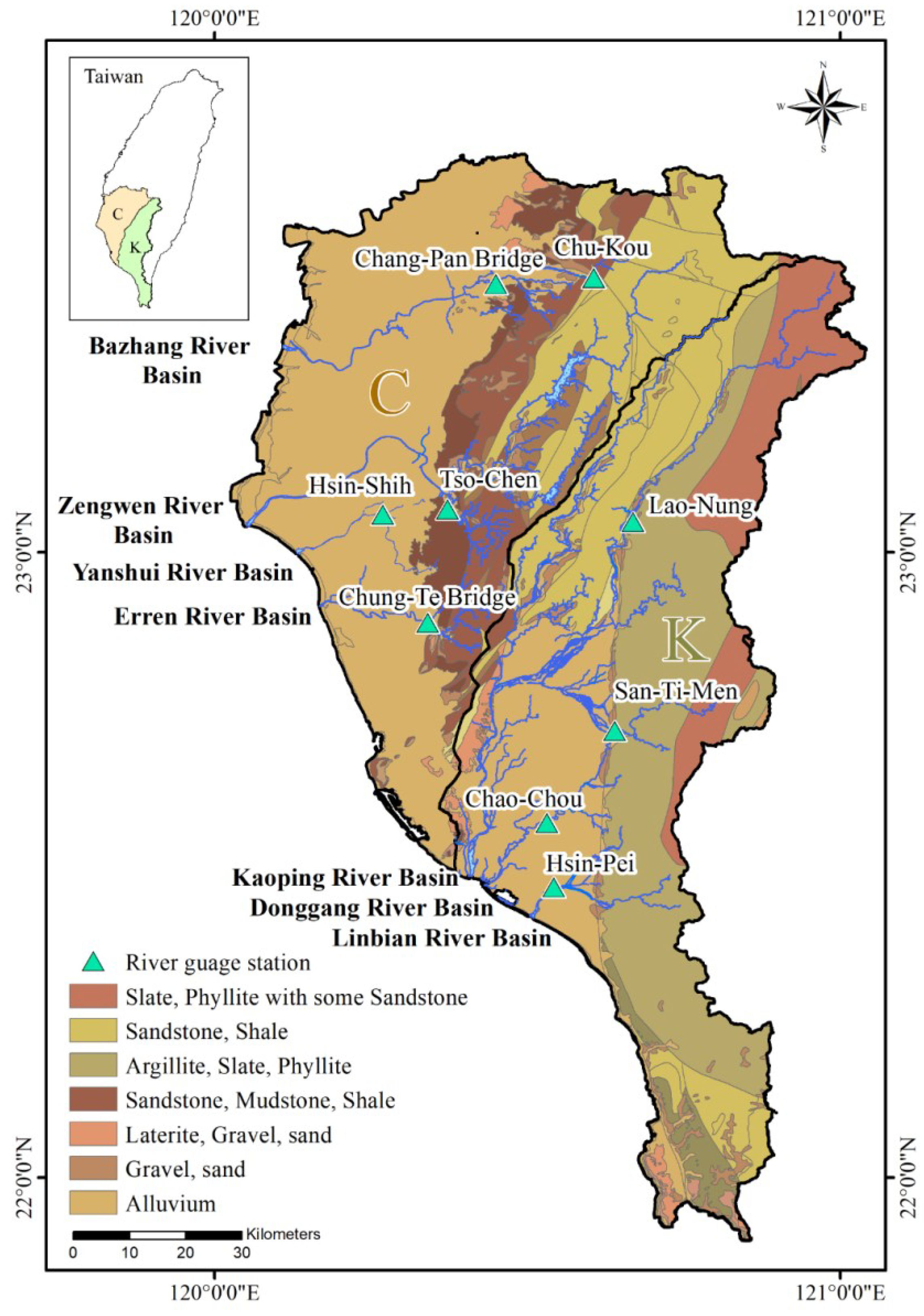
Southern Taiwan consists of several administrative divisions, including Chiayi County, Chiayi City, Tainan City, Kaohsiung City, and Pingtung County. The total area of the region is 10,002 km2, accounting for approximately 28% of the total area of Taiwan. Because of its tropical monsoonal climate, terrain, and geographical location, the rainy season is influenced by southwestern monsoons and typhoons from May to October. The dry season is influenced by northeastern monsoons from November to April and the leeward side causes less rainfall in this region [26]. The main rivers in the study area are the Bazhang, Zengwun, Yanshui, Erren, Kaoping, Donggang, and Linbian. In the present study, streamflow data from nine gauge stations in the catchments of Southern Taiwan were classified into dry season (November–April) and wet season (May–October) for the estimation of the respective catchment discharge characteristics and hydrogeological parameters during the dry and wet seasons. Table 1 shows information on the gauge stations in the catchments of Southern Taiwan.
Regarding the geological conditions of the study area, the Chianan Plain is primarily characterized by littoral and lagoon faces. Apart from a small number of areas with channel-fill deposits, there are no large fluvial deposits in the plain. On the North Chianan Plain, because of its slow sedimentation rates and longer emergent periods, there is an obviously weathered soil layer, and the relatively fine-grained sand accounts for a smaller proportion. On the South Chianan Plain, tectogenesis has divided the region into several separate underground zones by the consolidation of marine argillaceous strata. Although the sand layer accounts for a higher proportion of strata, the thicknesses of the sandy strata vary greatly because of tectonic influences. In addition, the widely distributed partially consolidated marine mudstone also reduces the lateral connectivity in the strata. These stratum characteristics result in low groundwater recharge from rainfall infiltration and, thereby, a shortage of groundwater resources on the Chianan Plain [28]. On the Pingtung Plain, metamorphism increases from west to east and the strata of the foothills, mainly consisting of black slate mixed with quartzite, contribute to the low permeability. The main aquifers within the plain are composed of unconsolidated rock, including older conglomerate alluvial fan deposits and, the most widely distributed, recent alluvium (Figure 1). The aquifers of the Pingtung Plain are well developed with relatively large thicknesses and a wide distribution. The thickness of the near-surface unconfined gravel aquifers decreases towards the west, with aquifuge thickness being much less than aquifer thickness. Within the plain, a continuous distribution of aquifuge only exists in the coastal areas [29]. According to reports of the differences in the spatial distribution of geology, we divided Southern Taiwan into the Chianan (Zengwun, Yanshui, and Erren river basins) and Kaoping (Kaoping, Donggang, and Linbian river basins) sub-areas in our discussion of the hydrogeology parameters.
3. Methodology
3.1. Low-Flow Recession Analysis Method
By utilizing the Boussinesq [30] hydrological model, for natural groundwater discharge from an unconfined aquifer into a channel, and the low-flow recession characteristics during no rainfall periods, and by assuming that evapotranspiration and internal flows within aquifers (excluding groundwater discharge) are negligible, Brutsaert and Nieber [12] proposed that a power relationship exists between streamflow (Q) and variation of streamflow (dQ/dt) under no-rainfall conditions, as shown in Equation (1):
where a and b are low-flow recession coefficients, and 1/a is equal to the e-folding time, also known as the characteristic time scale of the catchment discharge K (T) (i.e., the recession index). According to the previous study [31], when the streamflow at the start of the recession Q0 was used as the dimensionless discharge in the integration of Equation (1), the obtained recession index was highly correlated with 1/a. Therefore, in many subsequent studies, the recession index K has been applied in the explanation of nonlinear recession behavior. In the present study, the recession index was also investigated.
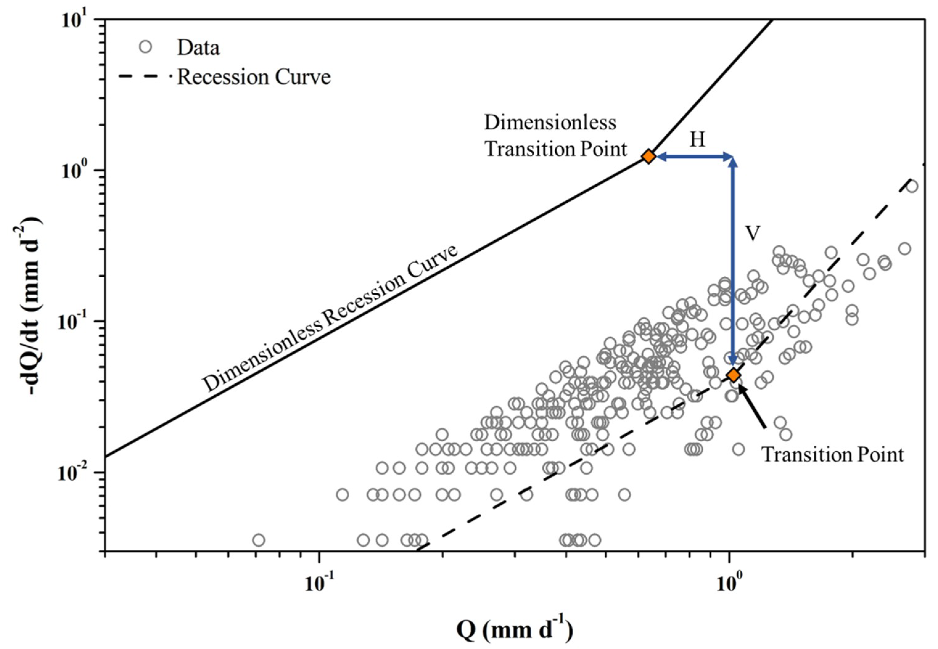
Assuming that the discharge behavior of an aquifer during the recession period is a function of the hydrogeological characteristics [32,33], by plotting the relationship between Q and dQ/dt and fitting the data to a recession curve, the catchment-scale aquifer characteristics can be indirectly estimated [14,34]. Under this concept, streamflow drainage from a catchment aquifer can be divided into two components: (1) a short-term flow regime that occurs when transient saturation exists in the aquifer for a short time after an initial rainfall event (b = 3) and (2) a long-term flow regime that involves the slower discharge of groundwater from the aquifer to the channel after rainfall infiltration (b = 1.5). These two flow regimes are characterized by their respective baseflow coefficients and constants. To appropriately assess the transition between the two flow regimes, Parlange et al. [35] proposed an analytical equation composed of the dimensionless discharge Q* and time t* for the theoretical dimensionless recession curve. Using this equation, the dimensionless transition point between the short-term and long-term regimes can be determined (log Q* = −0.1965, log (|dQ*/dt| = 0.0918)). By determining the horizontal placement (H) and vertical placement (V) between the transition point obtained from the recession analysis of the original data and the dimensionless transition point, the following equation can be used to estimate the catchment-scale hydrogeological parameters:
where Sy is the specific yield (-), k is the hydraulic conductivity (L/T), D is the saturated aquifer depth (L), A is the catchment area (L2), and B is the distance between the stream and the watershed (L) (B = A/2L, where L is the length of the main stream). However, it is difficult to clearly determine the actual location of the transitional point in the plot of dQ/dt vs. Q. Therefore, in this study, strategies proposed by Mendoza et al. [14] were adopted to locate three possible transition points to determine the range of values of the hydrogeological parameters in the catchment instead of using single values as representations of the respective characteristics. The placement strategies used to identify the transitional points are as follows:
- (1)
- First transition point: The intersection of the lower envelope lines of the short-term flow regime (b = 3) and long-term flow regime (b = 1.5) were defined through the application of the methodology proposed by Brutsaert and Nieber [12]. The envelope lines were placed such that 10% of the data points lay below the lines to reduce the influence of evapotranspiration.
- (2)
- Second transition point: The intersection of the linear regression line on the plot of dQ/dt vs. Q and the lower envelope for b = 3.
- (3)
- Third transition point: The intersection of the upper envelope for b = 1 and the highest log (Q) value among the data points.
The first transition point was determined based on past theoretical short-term and long-term flow regimes, the second transition point was determined by regarding the long-term flow regime as a representation of the overall variation in actual discharge, while the third transition point represents the maximum physical limit that may exist for the flow regime. Figure 2 shows that the dimensional recession curve translates to the recession curve with data in Q vs. −dQ/dt.
3.2. Selection Criteria for Recession Flow Data
The low-flow recession analysis method mainly involves the selection of recession time series record values from daily streamflow data and the plotting of the log–log graph of Q and dQ/dt for data fitting to achieve baseflow recession characteristic parameterization. Observed streamflow is composed of discharges such as surface runoff and interflow. As the low flow contributed by groundwater discharge has a lower recession rate compared to that of other discharges, to effectively select flows during recessions that constitute pure low flow, the selection of data points from raw data must fulfil certain criteria. In the present study, the following criteria proposed by Brutsaert [16] were used for data selection:
- (1)
- Eliminate all data points with positive and zero values of dQ/dt.
- (2)
- Eliminate two data points before dQ/dt becomes positive or zero, and three data points after the last positive and zero dQ/dt.
- (3)
- Eliminate four data points after major events, with major events defined based on the discharge duration curve [36].
- (4)
- Eliminate anomalous points in the data series.
- (5)
- Eliminate data points corresponding to days with daily rainfall >0 and several days after rainfall.
After data processing was performed using the selection criteria mentioned above, the selected data were used to plot the graph of dQ/dt vs. Q. Based on previous studies, a lower envelope line with a fixed gradient of b = 1 was used for data fitting for the definition of the baseflow coefficient a [16]. The lower envelope line was placed such that 10% of the data points lay below the line to eliminate the influence of evapotranspiration and ensure that the fit results reflected the discharge behavior constituted by low flow [37]. Lastly, the reciprocal relationship between the baseflow coefficient a and recession index K was used to calculate the recession index for the dry and wet seasons.
3.3. Recession-Curve-Displacement Method
The recession-curve-displacement method originated from the instantaneous recharge theory proposed by Rorabaugh [22], which describes the groundwater discharge per unit length of one side of the stream to the watershed q (L2) at a given time t, as shown in the following expansion formula:
where T is the transmissivity of the aquifer (L2/T), h0 is the instantaneous groundwater level rise (L), B is the distance between the stream and the watershed (L), and S is the storage coefficient (-). Assuming that small recharges can be neglected, Equation (3) can be simplified as follows:
The total groundwater discharge of the catchment Q (L3/T) can be determined from the product of the groundwater discharge q on both sides of the stream and the length of the main stream L (L) (, where A is the catchment area), as follows:
By applying the following model developed by Rorabaugh and Simons [38], the exponential function in Equation (4) can be replaced by the streamflow at a specific time:
where Qt is the peak flow of the recharge event and Q0 is the flow at the start of the recharge event.
By substituting Equations (4) and (6) into Equations (5) respectively, the following can be obtained:
Bevans [39] used the recession-curve-displacement method to calculate groundwater discharge. In this method, Equation (7) can be represented using the following formula:
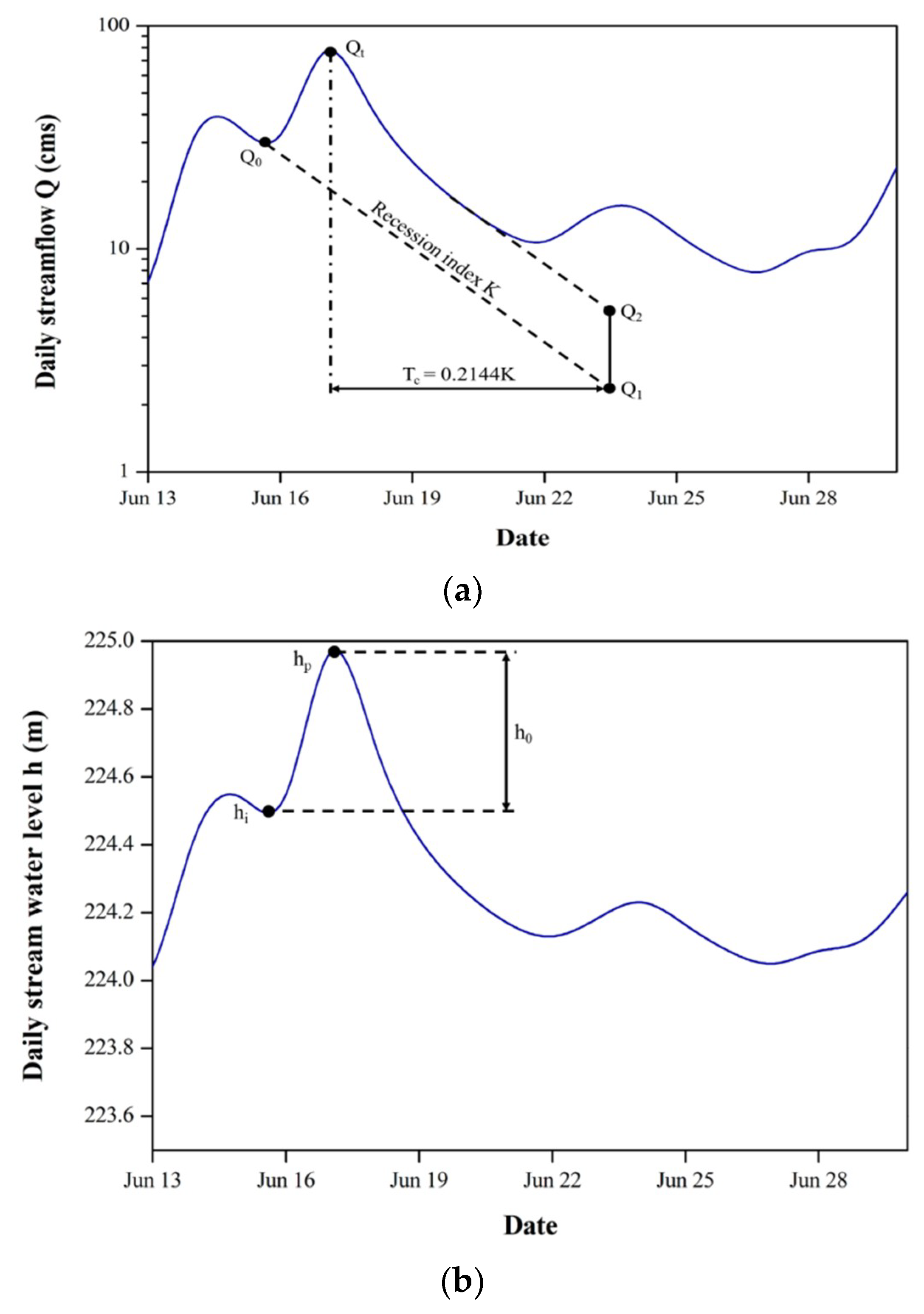
where Q2 is the theoretical groundwater discharge at a critical time Tc after the peak value of the recharge event, which is extrapolated from the post-event streamflow recession (L3/T); Q1 is the theoretical groundwater discharge at Tc extrapolated from the streamflow recession of the previous event (L3/T); K is the recession index of each log cycle (T) (also the characteristic drainage timescale); and Tc is the time from the peak to the end of infiltration recharge (i.e., linear recession) (T). Rorabaugh and Simons [38] defined the relationship between Tc and K as Tc = 0.2144K. From Equations (5) and (6), the formula for the estimated transmissivity of T can be obtained as follows:
When flow recession analysis methods have been used to estimate transmissivity, specific yield, and aquifer depth in previous studies, because of difficulties in solving the two equations in Equation (2) for the three unknown variables, the effective saturated aquifer depth, which undergoes variations at a smaller order of magnitude, was first typically estimated by multiplying the maximum potential aquifer depth (determined from the average elevation of the watersheds on both sides of the stream) by a proportionality constant. However, as this proportionality constant is related to the ratio of effective contribution by aquifer groundwater to the baseflow, which differs with different climatic, geographical and geological conditions, the definition of this constant is typically difficult, which leads to a high likelihood of overestimation or underestimation of effective aquifer depth. Therefore, the first step in the present study was to calculate the recession index K, which was subsequently input into the RORA program to determine Q0, Q1, Q2, and Qt in Equation (9) (refer to Figure 3). After obtaining the estimated transmissivity from further calculations, the transmissivity was directly proportional to the product of the hydraulic conductivity and the aquifer depth was used in combination with the equations for hydrogeological parameter estimation (Equation (2)) in the low-flow recession analysis method. This formed three equations with three unknowns, which could then be directly solved for the estimation of catchment-scale hydrogeological parameters.
4. Results and Discussion
4.1. Low-Flow Recession Analysis
In this study, the low-flow recession analysis method was used to estimate the recession index K, and to plot a graph of the flow variation (−dQ/dt) vs. flow (Q). Compared to the master recession curve method proposed by Barnes [40], this method avoids errors in the estimation of the transition point between direct runoff and low flow in the hydrograph [41] as well as the lack of representativeness of the reference point of a single event. The main assumption of this low-flow concept-based analysis method is the absence of rainfall and evapotranspiration influences. The selected data points are a discontinuous time series, therefore, the plot of dQ/dt vs. Q eliminates the uncertainty of the defined initial time and shows a discharge behavior that is representative of the entire catchment.
The results indicated that the average K values during the dry and wet seasons were 69.43 and 40.83 days, respectively. In particular, the result for the wet season was near the recession index of 45 ± 15 days for the large catchments reported by Brutsaert [16]. Table 2 shows the results of the recession index analysis. In general, K during the dry season was higher than that during the wet season for most catchments. This indicates that seasonal differences exist in the discharge regime of catchments in Southern Taiwan, which is consistent with the results of previous studies. For instance, in a study by Lyon et al. [42] on the variability of K within a valley in Tanzania, it was found that K showed higher variability in smaller, more upland catchments, while K values in larger, valley bottom catchments showed lower variability and were generally higher. This may be attributed to the fact that smaller catchments have a faster hydrological response than larger catchments, i.e., rainfall is rapidly reflected in aquifer discharge. As a result, different flow regimes exist during the dry and wet seasons, and this may also be associated with the influence of evapotranspiration. Because of differences in vertical flow in the aquifers during the dry and wet seasons, the variability of K is higher. Although a previous study [43] asserted that evapotranspiration has a limited influence on the baseflow coefficient, considering that Southern Taiwan and Tanzania have highly similar seasonal climates and higher potential evapotranspiration during summer, the existence of seasonal differences in the recession index K in Southern Taiwan is reasonable. Notably, the high and low values of the recession index may well result from influences on vegetation and soil properties; for instance, reduced vegetation cover or poorer soil permeability may lead to reduced groundwater evapotranspiration, thus resulting in a reduced low-flow recession rate. The in-depth investigation of the possible influencing factors has not been included in the scope of this study as it requires the use of other methods such as groundwater tracers.
4.2. Estimation of Hydrogeological Parameters
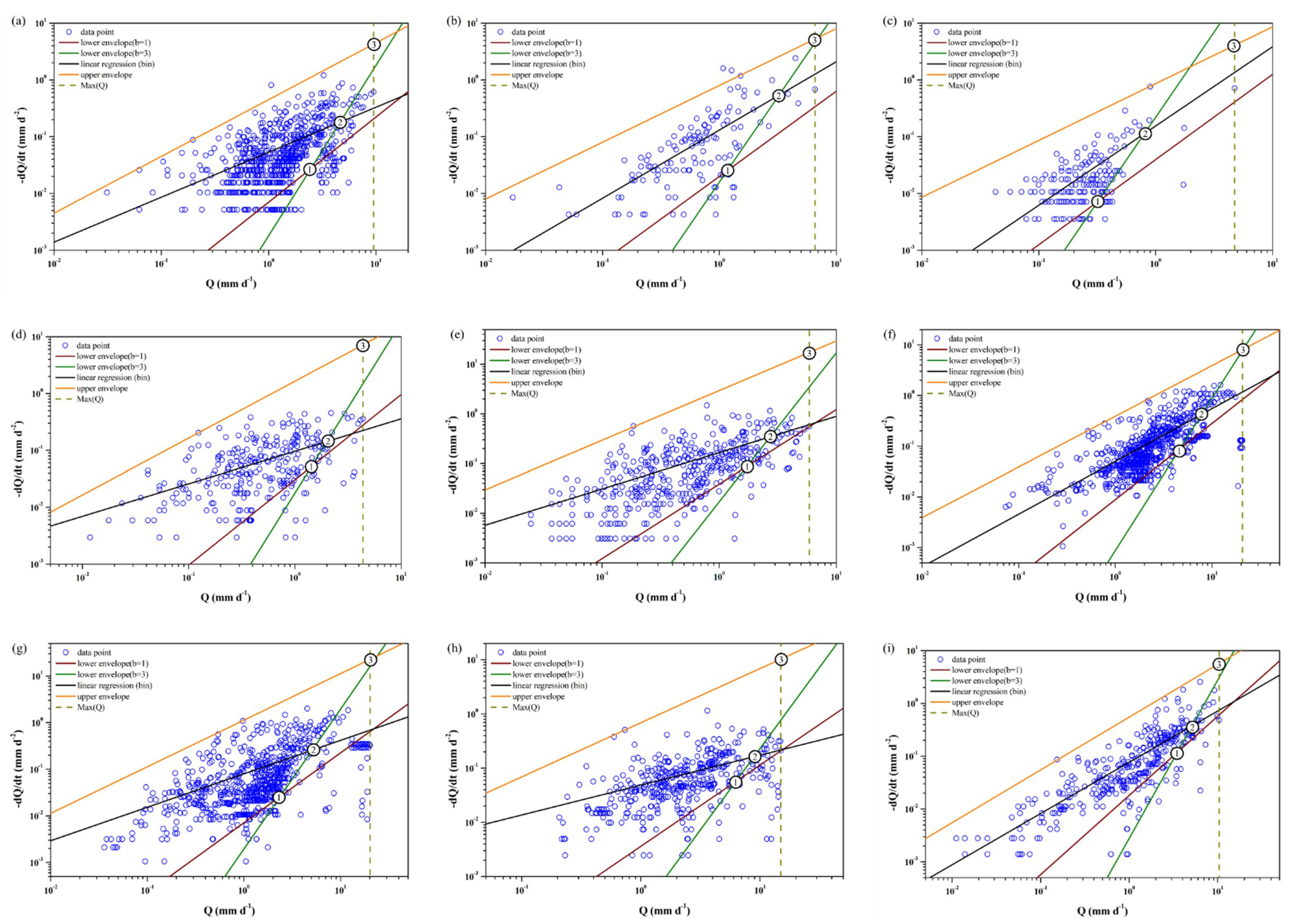
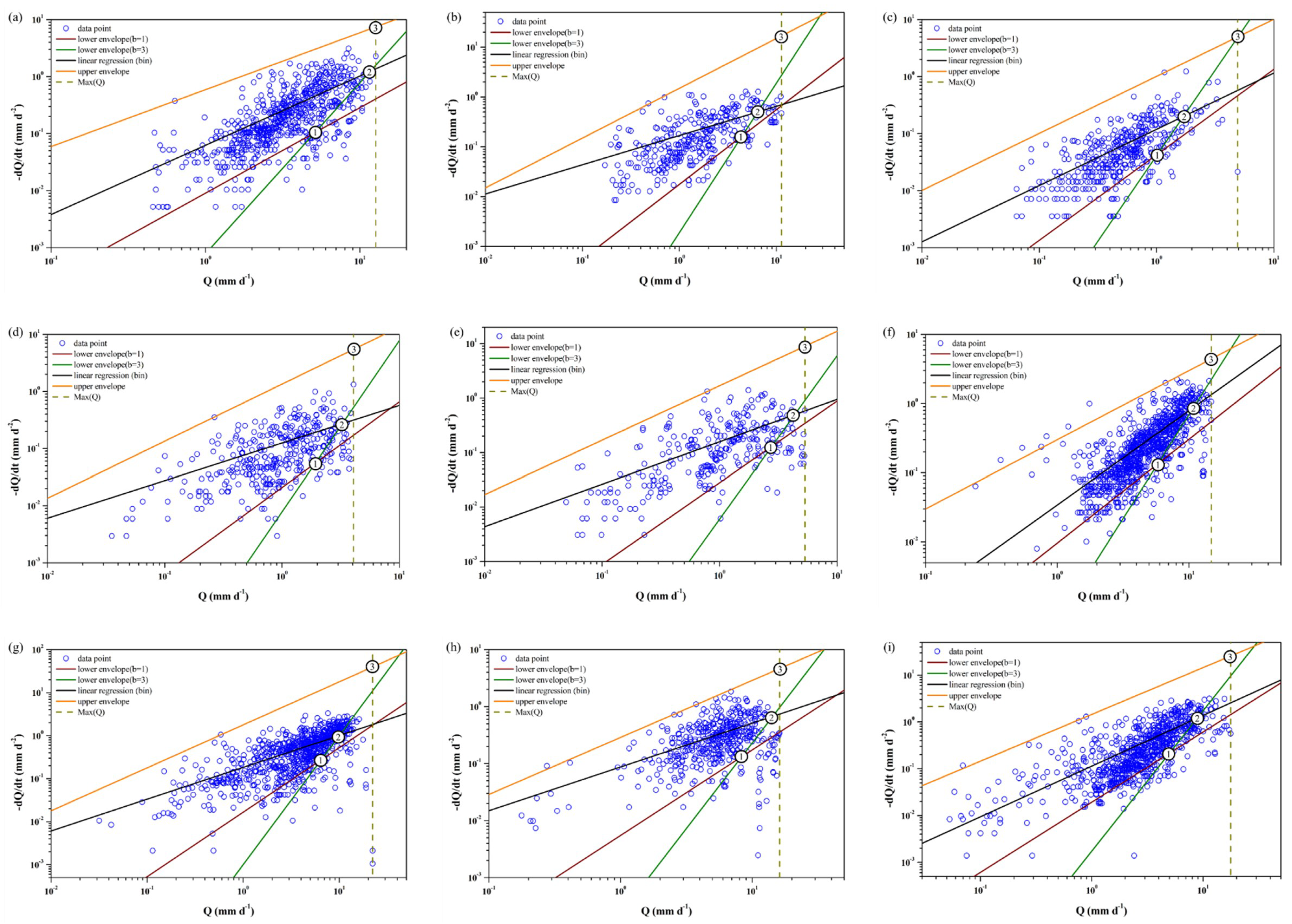
In previous studies that utilized flow recession analysis methods for the estimation of hydrogeological parameters, an initial estimate of the effective aquifer depth was usually required at the beginning of the estimation process. This initial estimate was typically obtained by multiplying the maximum potential aquifer depth D (average elevation of watersheds on both sides of the stream), determined using satellite or aerial image data by a proportionality constant, which was associated with the aquifer groundwater contribution to baseflow. However, the aquifer groundwater contribution to baseflow cannot be quantified based on the discharge characteristics of the catchment, the different values of this constant may lead to significant differences in the estimation results of the hydrogeological parameters. Therefore, our study adopted a combination of the low-flow recession analysis method, which was used to estimate the effective aquifer depth D, specific yield Sy, and hydraulic conductivity k, and the recession-curve-displacement method, which was used to estimate the transmissivity T. Based on the fact that transmissivity is directly proportional to the product of hydraulic conductivity and effective aquifer depth, direct calculations could be performed to obtain estimates of transmissivity, hydraulic conductivity, and specific yield. This approach effectively eliminated the subjectivity involved in the determination of the proportionality constant for the initial estimation of effective aquifer depth. To evaluate hydrogeological parameters, the three transition points were determined by a regression line and envelopes in the graph of Q vs. –dQ/dt to calculate the placement with the dimensionless transition points. Figure 4 and Figure 5 show the transition points of dry and wet seasons determined by the low-flow recession method in each catchment. Lastly, the estimation results were compared to those of field tests.
As the field test results consisted of separate results for the Chianan and Pingtung plains, the results of the present study were also classified for either the Chianan sub-area (Zengwun, Yanshui, and Erren river basins) or for the Kaoping sub-area (Kaoping, Donggang, and Linbian river basins). Estimations were conducted based on the second transition point, which has been commonly used in previous studies, and the median values of the estimation results were selected to represent the catchment-scale hydrogeological parameters. Table 3 shows a comparison of the estimation and field test results. In particular, the specific yield values obtained from field tests in the Chianan sub-area were not referenced as there were only two boreholes in the region. However, the other results indicated small differences in the estimated hydrogeological parameter values during the dry and wet seasons for both the Chianan and Kaoping sub-areas. This could be because of differences in the properties of aquifers that are passed through by groundwater in the dry and wet seasons. In addition, as field tests were conducted at the local scale while estimations in our study yielded catchment-scale parameters, the difference in scale may have also led to slight differences between the field test and estimation results.
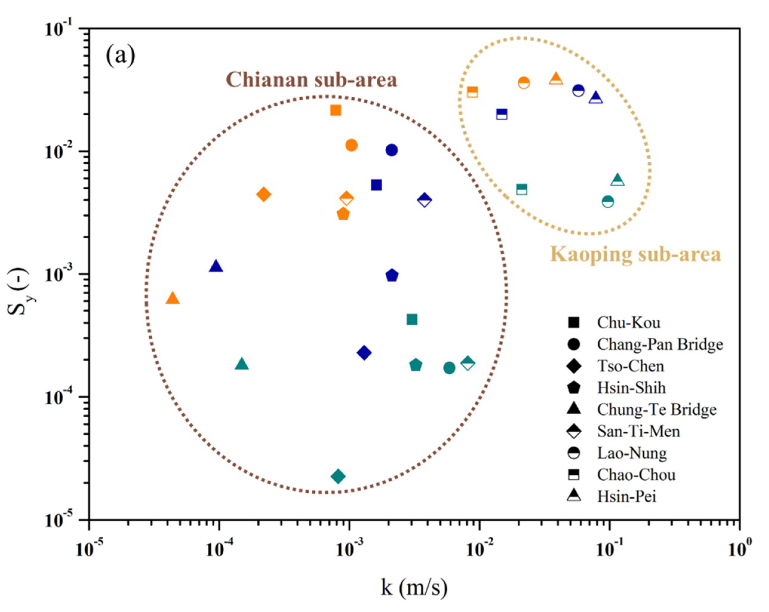
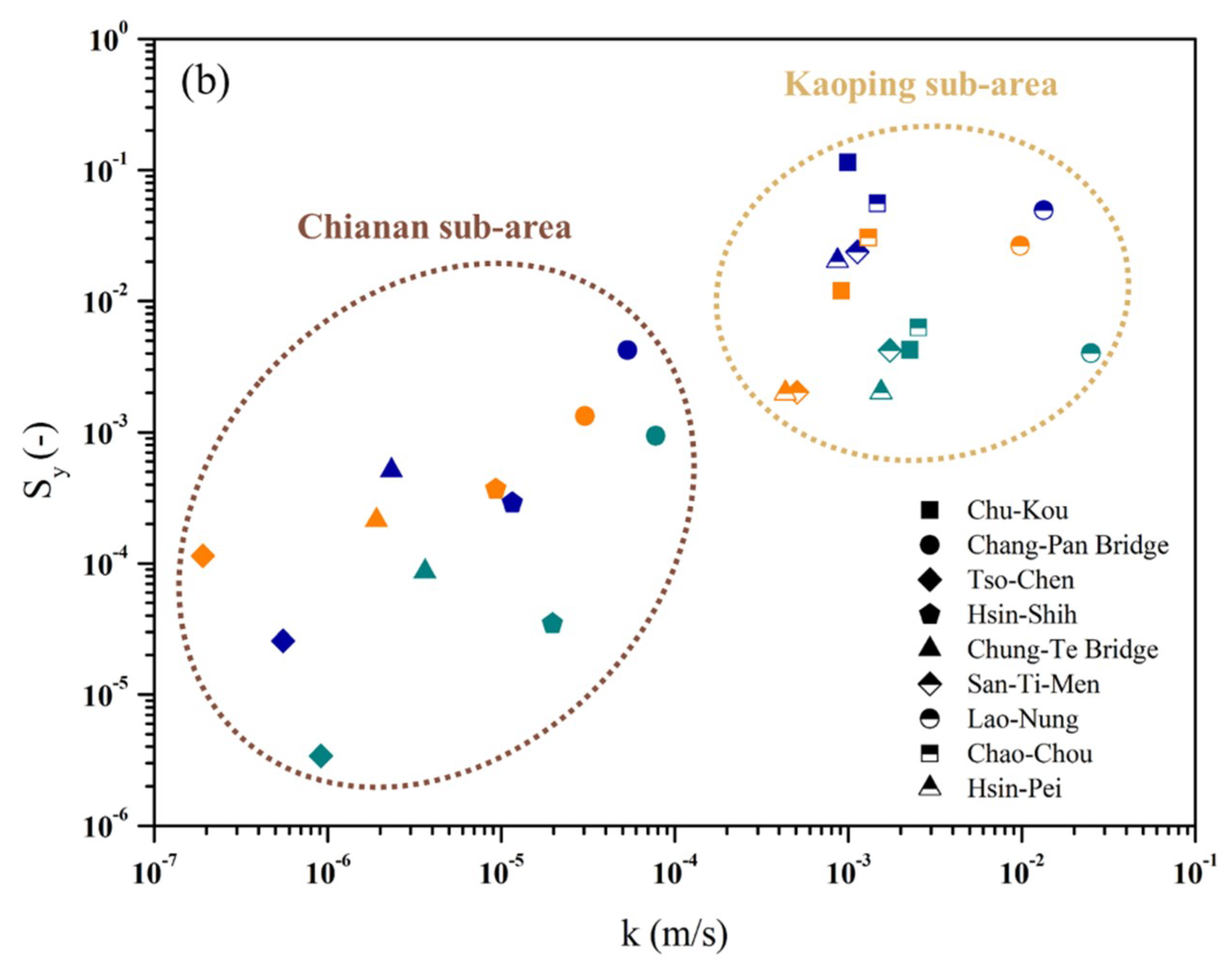
To determine if regional differences were visible in the hydrogeological parameters, graphs of hydraulic conductivity vs. specific yield for different transition points during the dry and wet seasons were plotted, as shown in Figure 6. The graphs showed that differences existed in the hydrogeological parameters of the Chianan and Kaoping sub-areas during both the dry and wet seasons and at different transition points. This indicates the presence of regional differences in the estimated parameters, which was consistent with the distribution of geological structures in Southern Taiwan (refer to Figure 1). As shown in the diagram of the study area, although the soil of the middle and lower reaches of the Chianan and Kaoping sub-areas consists primarily of alluvial soil, the upper reaches of the Chianan sub-area contain mudstone, which has poorer permeability. In addition, aquifers of the South and North Chianan plains have reduced connectivity and permeability because of the respective influences of geological structures and a weathered soil horizon. In contrast, the aquifers in the Kaoping sub-area are of greater depth and are less affected by tectogenesis. These characteristics may have led to lower estimated values of hydraulic conductivity and specific yield in the Chianan sub-area compared to those of the Kaoping sub-area. However, for the San-Ti-Men gauging station in the Kaoping sub-area, the obtained results were particularly intriguing. The estimated values of the hydrogeological parameters during the wet season were similar to those of the Kaoping sub-area, while the estimated values during the dry season were similar to those of the Chianan sub-area. The main reason might have been that groundwater passed through fewer aquifers during the dry season compared to the wet season, which resulted in lower estimated values during the dry season. The ranges of estimated values for the hydrogeological parameters of the four gauge stations in the Chianan sub-area, because of differences in geological structure between the North and South Chianan plains, were larger than those of the Kaoping sub-area. The results also showed that the southern region of the Chianan sub-area has a higher proportion of sand strata but smaller estimated values for the hydrogeological parameters. This could be because tectogenesis has led to lower lateral connectivity. This has resulted in significantly lower estimated values on the catchment scale of the southern region than that of the northern region of the Chianan sub-area, which has a lower proportion of sand strata. From the aforementioned results, it is apparent that the present study was not only successful in estimating the hydrogeological parameters but also enabled an understanding of the overall discharge behavior through the use of the recession index. It validated the differences in the distribution of geological structures in the different regions through the analysis of the estimated hydrogeological parameters. The results of the present study may be used as a reference point for future constructions of hydrological or relevant physical models and for decisions concerning water resources management.
5. Conclusions
In the present study, a combination of the low-flow recession analysis method, which is based on the water balance in hydrological systems, and the recession-curve-displacement method, which is based on streamflow hydrographs, was used for the estimation of hydrogeological parameters of catchments in Southern Taiwan. The recession index K derived from the low-flow recession analysis method was used to determine the seasonal differences in the discharge regimes of aquifers in the catchments. Subsequently, the respective estimation results for transmissivity T, hydraulic conductivity k, and specific yield Sy for the dry and wet seasons were compared to the results of field tests. The comparison results indicated small differences between the estimation results for the dry and wet seasons as well as slight differences in the local-scale and catchment-scale hydrogeological parameters. The graphs of hydraulic conductivity vs. specific yield showed significant regional differences and consistency with the distribution of geological structures. They demonstrated the applicability and representativeness of the low-flow recession analysis method in the estimation of hydrogeological parameters. The present study differs from costly field tests, which merely produce local-scale results for the estimation of hydrogeological parameters, because hydrological data that could be readily acquired and were representative of catchment discharge behavior were used. A combination of two flow recession analysis methods was employed to eliminate subjectivity in the initial estimation of one parameter, a problem that has frequently been encountered in previous studies. The estimated catchment-scale hydrogeological parameters demonstrated that flow recession analysis can provide a rapid, low-cost, and effective means of estimating hydrogeological parameters, which can facilitate the construction of future hydrological models and a better understanding of the role of groundwater in various catchments or basins of Taiwan in the hydrological cycle. They can also serve as a reference for decisions regarding groundwater resource management under conditions of climate change.
Author Contributions
C.-C.H. contrived the subject of the article, performed the literature review and contributed to the writing of the paper; H.-F.Y. participated in data processing and the elaboration of the statistical analysis and figures.
Funding
This research was funded by the Research Project of the Ministry of Science and Technology (MOST), grant number (107-2116-M-006-011).
Acknowledgments
The authors are grateful for the support from the Headquarters of University Advancement at the National Cheng Kung University, sponsored by the Ministry of Education, Taiwan, ROC.
Conflicts of Interest
The authors declare no conflicts of interest.
References
- Alley, W.; Healy, R.; LaBaugh, J.; Reilly, T. Hydrology—Flow and storage in groundwater systems. Science 2002, 296, 1985–1990. [Google Scholar] [CrossRef] [PubMed]
- Xu, C.Y.; Singh, V.P. Review on regional water resources assessment models under stationary and changing climate. Water Resour. Manag. 2004, 18, 591–612. [Google Scholar] [CrossRef]
- Conama, D. Estudio de la Variabilidad Climática en Chile Para el Siglo XXI; Departamento de Geofısica, Universidad de Chile: Santiago, Chile, 2006. [Google Scholar]
- Berghuijs, W.R.; Hartmann, A.; Woods, R.A. Streamflow sensitivity to water storage changes across Europe. Geophys. Res. Lett. 2016, 43, 1980–1987. [Google Scholar] [CrossRef]
- Staudinger, M.; Stoelzle, M.; Seeger, S.; Seibert, J.; Weiler, M.; Stahl, K. Catchment water storage variation with elevation. Hydrol. Process. 2017, 31, 2000–2015. [Google Scholar] [CrossRef]
- Lin, K.T.; Yeh, H.F. Baseflow recession characterization and groundwater storage trends in northern Taiwan. Hydrol. Res. 2017. [Google Scholar] [CrossRef]
- Oyarzún, R.; Godoy, R.; Núñez, J.; Fairley, J.P.; Oyarzún, J.; Maturana, H.; Freixas, G. Recession flow analysis as a suitable tool for hydrogeological parameter determination in steep, arid basins. J. Arid Environ. 2014, 105, 1–11. [Google Scholar] [CrossRef]
- Vannier, O.; Braud, I.; Anquetin, S. Regional estimation of catchment—Scale soil properties by means of streamflow recession analysis for use in distributed hydrological models. Hydrol. Process. 2014, 28, 6276–6291. [Google Scholar] [CrossRef]
- Arumí, J.L.; Maureira, H.; Souvignet, M.; Pérez, C.; Rivera, D.; Oyarzún, R. Where does the water go? Understanding geohydrological behaviour of Andean catchments in south-central Chile. Hydrol. Sci. J. 2016, 61, 844–855. [Google Scholar] [CrossRef]
- Senkondo, W.; Tuwa, J.; Koutsouris, A.; Lyon, S.W. Estimating Aquifer Transmissivity Using the Recession-Curve-Displacement Method in Tanzania’s Kilombero Valley. Water 2017, 9, 948. [Google Scholar] [CrossRef]
- Smakhtin, V.U. Low flow hydrology: A review. J. Hydrol. 2001, 240, 147–186. [Google Scholar] [CrossRef]
- Brutsaert, W.; Nieber, J.L. Regionalized drought flow hydrographs from a mature glaciated plateau. Water Resour. Res. 1977, 13, 637–643. [Google Scholar] [CrossRef]
- Roques, C.; Rupp, D.E.; Selker, J.S. Improved streamflow recession parameter estimation with attention to calculation of −dQ/dt. Adv. Water Resour. 2017, 108, 29–43. [Google Scholar] [CrossRef]
- Mendoza, G.F.; Steenhuis, T.S.; Walter, M.T.; Parlange, J.Y. Estimating basin-wide hydraulic parameters of a semi-arid mountainous watershed by recession-flow analysis. J. Hydrol. 2003, 279, 57–69. [Google Scholar] [CrossRef]
- Dewandel, B.; Lachassagne, P.; Bakalowicz, M.; Weng, P.H.; Al-Malki, A. Evaluation of aquifer thickness by analysing recession hydrographs. Application to the Oman ophiolite hard-rock aquifer. J. Hydrol. 2003, 274, 248–269. [Google Scholar] [CrossRef]
- Brutsaert, W. Long-term groundwater storage trends estimated from streamflow records: Climatic perspective. Water Resour. Res. 2008, 44, W02409. [Google Scholar] [CrossRef]
- Sawaske, S.R.; Freyberg, D.L. An analysis of trends in baseflow recession and low-flows in rain-dominated coastal streams of the pacific coast. J. Hydrol. 2014, 519, 599–610. [Google Scholar] [CrossRef]
- Stoelzle, M.; Stahl, K.; Weiler, M. As simple as possible? Drought recognition based on streamflow recession. In Proceedings of the 10th International Conference on Hydroinformatics, Hamburg, Germany, 14–18 July 2012; pp. 1–8. [Google Scholar]
- Stoelzle, M.; Stahl, K.; Morhard, A.; Weiler, M. Streamflow sensitivity to drought scenarios in catchments with different geology. Geophys. Res. Lett. 2014, 41, 6174–6183. [Google Scholar] [CrossRef] [Green Version]
- Van Dijk, A.I.J.M. Climate and terrain factors explaining streamflow response and recession in Australian catchments. Hydrol. Earth Syst. Sci. 2010, 14, 159–169. [Google Scholar] [CrossRef]
- Beck, H.E.; Dijk, A.I.; Miralles, D.G.; Jeu, R.A.; McVicar, T.R.; Schellekens, J. Global patterns in base flow index and recession based on streamflow observations from 3394 catchments. Water Resour. Res. 2013, 49, 7843–7863. [Google Scholar] [CrossRef] [Green Version]
- Rorabough, M.I. Estimating changes in bank storage and grounwater contribution to streamflow. Int. Assoc. Sci. Hydrol. Publ. 1964, 63, 432–441. [Google Scholar]
- Abo, R.K.; Merkel, B.J. Investigation of the potential surface–groundwater relationship using automated base-flow separation techniques and recession curve analysis in Al Zerba region of Aleppo, Syria. Arab. J. Geosci. 2015, 8, 10543–10563. [Google Scholar] [CrossRef]
- Rutledge, A.T. Computer Programs for Describing the Recession of Ground-Water Discharge and for Estimating mean Ground-Water Recharge and Discharge from Streamflow Record; U.S. Geological Survey, U.S.G.S. Earth Science Information Center, Open-File Reports Section: Reston, VA, USA, 1993.
- Zhang, L.; Brutsaert, W.; Crosbie, R.; Potter, N. Long-term annual groundwater storage trends in Australian catchments. Adv. Water Resour. 2014, 74, 156–165. [Google Scholar] [CrossRef]
- Water Resources Agency. Hydrological Year Book; Water Resources Agency: Taipei, Taiwan, 2017. (In Chinese) [Google Scholar]
- Water Resources Agency. The Third Stage Management Project of Climate Change Impacts and Adaptation on Water Environment (3/5); Water Resources Agency: Taipei, Taiwan, 2016. (In Chinese) [Google Scholar]
- Water Resources Agency. Assessment of Groundwater Potential Exploiting Zones and Groundwater Yields in Kaoping and Chianan Watersheds (2/2); Water Resources Agency: Taipei, Taiwan, 2017. (In Chinese) [Google Scholar]
- Central Geological Survey. Hydrogeology Investigation and Groundwater Resource Assessment for Taiwan-Groundwater Recharge Estimation amd Model Simulation Pingtung Plain; Central Geological Survey: Taipei, Taiwan, 2012. (In Chinese) [Google Scholar]
- Boussinesq, J. Essai sur la théorie des eaux courantes. Imprimerie Nationale: Paris, France, 1877.
- Bogaart, P.W.; Van Der Velde, Y.; Lyon, S.W.; Dekker, S.C. Streamflow recession patterns can help unravel the role of climate and humans in landscape co-evolution. Hydrol. Earth Syst. Sci. 2016, 20, 1413–1432. [Google Scholar] [CrossRef] [Green Version]
- Rupp, D.E.; Selker, J.S. On the use of the Boussinesq equation for interpreting recession hydrographs from sloping aquifers. Water Resour. Res. 2006, 42, W12421. [Google Scholar] [CrossRef]
- Zhang, L.; Chen, Y.D.; Hickel, K.; Shao, Q. Analysis of low-flow characteristics for catchments in Dongjiang Basin, China. Hydrogeol. J. 2009, 17, 631–640. [Google Scholar] [CrossRef]
- Szilagyi, J. Vadose zone influences on aquifer parameter estimates of saturated-zone hydraulic theory. J. Hydrol. 2004, 286, 78–86. [Google Scholar] [CrossRef] [Green Version]
- Parlange, J.Y.; Stagnitti, F.; Heilig, A.; Szilagyi, J.; Parlange, M.B.; Steenhuis, T.S.; Hogarth, W.L.; Barry, D.A.; Li, L. Sudden drawdown and drainage of a horizontal aquifer. Water Resour. Res. 2001, 37, 2097–2101. [Google Scholar] [CrossRef] [Green Version]
- Kingsford, R.T.; Thomas, R.F. Environmental Flows on the Paroo and Warrego Rivers; National Parks & Wildlife Service: New South Wales, Australia, 2000. [Google Scholar]
- Troch, P.A.; Mancini, M.; Paniconi, C.; Wood, E.F. Evaluation of a distributed catchment scale water balance model. Water Resour. Res. 1993, 29, 1805–1817. [Google Scholar] [CrossRef] [Green Version]
- Rorabaugh, M.I.; Simons, W.D. Exploration of Methods of Relating Ground Water to Surface Water, Columbia River Basin-Second Phase: U.S. Geol. Survey (USGS) Open-File Report; US Geological Survey: Reston, VA, USA, 1966. [Google Scholar]
- Bevans, H.E. Estimating Stream-Aquifer Interactions in Coal Areas of Eastern Kansas by Using Streamflow Records; US Geological Survey Water Supply Paper; US Geological Survey: Reston, VA, USA, 1986; pp. 51–64.
- Barnes, B.S. The structure of discharge-recession curves. Eos Trans. Am. Geophys. Union 1939, 20, 721–725. [Google Scholar] [CrossRef]
- Anderson, M.G.; Burt, T.P. Interpretation of recession flow. J. Hydrol. 1980, 46, 89–101. [Google Scholar] [CrossRef]
- Lyon, S.W.; Koutsouris, A.; Scheibler, F.; Jarsjö, J.; Mbanguka, R.; Tumbo, M.; Robert, K.K.; Sharma, A.N.; van der Velde, Y. Interpreting characteristic drainage timescale variability across Kilombero Valley, Tanzania. Hydrol. Process. 2015, 29, 1912–1924. [Google Scholar] [CrossRef]
- Shaw, S.B.; McHardy, T.M.; Riha, S.J. Evaluating the influence of watershed moisture storage on variations in base flow recession rates during prolonged rain-free periods in medium-sized catchments in New York and Illinois, USA. Water Resour. Res. 2013, 49, 6022–6028. [Google Scholar] [CrossRef] [Green Version]
Figure 1.
Spatial distribution of gauge stations and geological map of Southern Taiwan. C—Chianan sub-area; K—Kaoping sub-area.
Figure 1.
Spatial distribution of gauge stations and geological map of Southern Taiwan. C—Chianan sub-area; K—Kaoping sub-area.

Figure 2.
The dimensionless recession curve and dimensionless transition point are translated to the recession curve and transition point with data. Horizontal placement (H) and vertical placement (V) are also identified above.
Figure 2.
The dimensionless recession curve and dimensionless transition point are translated to the recession curve and transition point with data. Horizontal placement (H) and vertical placement (V) are also identified above.

Figure 3.
A schematic diagram of the displacement-curve-displacement method with the definition of (a) Q0, Qt, Q1, and Q2 and (b) h0 (hi and hp are the streamflow water level corresponding to Q0 and Qt respectively).
Figure 3.
A schematic diagram of the displacement-curve-displacement method with the definition of (a) Q0, Qt, Q1, and Q2 and (b) h0 (hi and hp are the streamflow water level corresponding to Q0 and Qt respectively).

Figure 4.
The relationship between Q and –dQ/dt for each catchment in dry seasons. Three transition points are indicated with the regression line and envelopes and showed as circles with number. (a) Chu-Kou, (b) Chang-Pan Bridge, (c) Tso-Chen, (d) Hsin-Shih, (e) Chung-Te Bridge, (f) Lao-Nung, (g) San-Ti-Men, (h) Chao-Chou, and (i) Hsin-Pei.

Figure 5.
The relationship between Q and –dQ/dt for each catchment in wet seasons. Three transition points are indicated with the regression line and envelopes and showed as circles with number. (a) Chu-Kou, (b) Chang-Pan Bridge, (c) Tso-Chen, (d) Hsin-Shih, (e) Chung-Te Bridge, (f) Lao-Nung, (g) San-Ti-Men, (h) Chao-Chou, and (i) Hsin-Pei.

Figure 6.
Hydraulic conductivity k vs. specific yield Sy at different transition points in Southern Taiwan. The shapes of symbols represent each station, and transition points 1, 2 and 3 are green, blue and orange symbols, respectively. (a) Dry season; (b) wet season.
Figure 6.
Hydraulic conductivity k vs. specific yield Sy at different transition points in Southern Taiwan. The shapes of symbols represent each station, and transition points 1, 2 and 3 are green, blue and orange symbols, respectively. (a) Dry season; (b) wet season.


Table 1.
Information on gauge stations in Southern Taiwan.
| Basin | Station | Area (km2) | X-Coordinate (TWD67 a) | Y-Coordinate (TWD67 a) | Record Years |
|---|---|---|---|---|---|
| Bazhang River | Chu-Kou | 83.1 | 209,775.8 | 2,592,901.4 | 1967–2017 |
| Chang-Pan Bridge | 101.1 | 193,794.3 | 2,591,889.4 | 1970–2017 | |
| Zengwen River | Tso-Chen | 121.3 | 186,554.1 | 2,551,818.6 | 1971–2017 |
| Yanshui River | Hsin-Shih | 146.5 | 175,903.5 | 2,550,924.6 | 1973–2017 |
| Erren River | Chung-Te Bridge | 139.6 | 183,217.2 | 2,531,714.6 | 1982–2017 |
| Kaoping River | Lao-Nung | 812.0 | 216,098.8 | 2,549,698.6 | 1959–2008 |
| San-Ti-Men | 408.5 | 213,804.4 | 2,512,457.7 | 1964–2017 | |
| Donggang River | Chao-Chou | 175.3 | 203,071.1 | 2,496,579.8 | 1965–2017 |
| Linbian River | Hsin-Pei | 309.9 | 203,708 | 2,484,782.9 | 1962–2013 |
Note: a is Taiwan’s Triangulation Point Coordinates.
Table 2.
Recession index K of dry and wet seasons in Southern Taiwan.
| Station | K | |
|---|---|---|
| Dry Season | Wet Season | |
| Chu-Kou | 117.65 | 57.80 |
| Chang-Pan Bridge | 50 | 30.30 |
| Tso-Chen | 51.81 | 31.45 |
| Hsin-Shih | 39.53 | 37.45 |
| Chung-Te Bridge | 29.94 | 31.25 |
| Lao-Nung | 70.42 | 55.56 |
| San-Ti-Men | 93.76 | 29.85 |
| Chao-Chou | 131.58 | 58.82 |
| Hsin-Pei | 40.16 | 34.97 |
| Chu-Kou | 69.43 | 40.83 |
Table 3.
Hydrogeological parameters of pumping test and estimates using the flow recession method in the Chianan and Kaoping sub-areas.
Table 3.
Hydrogeological parameters of pumping test and estimates using the flow recession method in the Chianan and Kaoping sub-areas.
| Chianan Sub-Area | |||
| Hydrogeological Parameters | Pumping Test | Dry Season | Wet Season |
| T (m2/min) | 2.63 × 10⁻¹–4.40 × 10⁻³ | 100–10−2 | 100–10−2 |
| k (m/s) | 10−4–10−6 | 10−3–10−5 | 10−4–10−6 |
| Sy (-) | 10−2 | 10−2–10−4 | 10−1–10−5 |
| Kaoping Sub-Area | |||
| Hydrogeological Parameters | Pumping Test | Dry Season | Wet Season |
| T (m/min) | 3.00 × 10⁻⁵–1.51 × 101 | 100–101 | 100 |
| k (m/s) | 10−3–10−5 | 10−2–10−3 | 10−2–10−3 |
| Sy (-) | 10−1–10−5 | 10−2–10−3 | 10−2 |
© 2018 by the authors. Licensee MDPI, Basel, Switzerland. This article is an open access article distributed under the terms and conditions of the Creative Commons Attribution (CC BY) license (http://creativecommons.org/licenses/by/4.0/).
Share and Cite
MDPI and ACS Style
Huang, C.-C.; Yeh, H.-F. Hydrogeological Parameter Determination in the Southern Catchments of Taiwan by Flow Recession Method. Water 2019, 11, 7. https://doi.org/10.3390/w11010007
AMA Style
Huang C-C, Yeh H-F. Hydrogeological Parameter Determination in the Southern Catchments of Taiwan by Flow Recession Method. Water. 2019; 11(1):7. https://doi.org/10.3390/w11010007
Chicago/Turabian StyleHuang, Chia-Chi, and Hsin-Fu Yeh. 2019. "Hydrogeological Parameter Determination in the Southern Catchments of Taiwan by Flow Recession Method" Water 11, no. 1: 7. https://doi.org/10.3390/w11010007
Note that from the first issue of 2016, this journal uses article numbers instead of page numbers. See further details here.