Evaluation of Return Period and Risk in Bivariate Non-Stationary Flood Frequency Analysis

Abstract

The concept of a traditional return period has long been questioned in non-stationary studies, and the risk of failure was recommended to evaluate the design events in flood modeling. However, few studies have been done in terms of multivariate cases. To investigate the impact of non-stationarity on the streamflow series, the Yichang station in the Yangtze River was taken as a case study. A time varying copula model was constructed for bivariate modeling of flood peak and 7-day flood volume, and the non-stationary return period and risk of failure were applied to compare the results between stationary and non-stationary models. The results demonstrated that the streamflow series at the Yichang station showed significant non-stationary properties. The flood peak and volume series presented decreasing trends in their location parameters and the dependence structure between them also weakened over time. The conclusions of the bivariate non-stationary return period and risk of failure were different depending on the design flood event. In the event that both flood peak and volume are exceeding, the flood risk is smaller with the non-stationary model, which is a joint effect of the time varying marginal distribution and copula function. While in the event that either flood peak or volume exceed, the effect of non-stationary properties is almost negligible. As for the design values, the non-stationary model is characterized by a higher flood peak and lower flood volume. These conclusions may be helpful in long-term decision making in the Yangtze River basin under non-stationary conditions.

1. Introduction

A flood is a natural hazard that may cause great damages to human civilization, and it is studied worldwide using hydrologic as well as hydraulic models [1,2]. Flood frequency analysis, a commonly used method in hydrological modeling, has been applied in the calculation of various design values, such as dams, bridges, culverts and many other hydraulic constructions [3,4]. However, the flood frequency analysis is based on some assumptions in terms of statistics, one of which is the well-known stationary assumption. As climate change and human activities intensify, the stationary assumption has faced more and more challenges [5]. Much research has been done to study the non-stationarity in a hydrological series. For example, Zhang et al. [6] used three methods to investigate the effect of dams and lakes on the streamflow series in the Yangtze River basin. Ishak et al. [7] used a regional Mann-Kendall test to explore the non-stationary properties in annual maximum flood series for 491 catchments in Australia. O’Brien and Burn [8] used a non-stationary index-flood technique to estimate the extreme quantiles of annual maximum streamflow. Most of the studies supported the proposition by Milly et al. [5] and concluded that a non-stationary modeling framework may provide valuable information for policy implementation and hazard prevention.

The return period is an important indicator of risk for a design flood event; however, in the context of non-stationary, it may conceal the actual meaning of underlying mechanism [9] and even lead to misconceptions. To tackle such problems, its concept has been reformulated and extended to accommodate the non-stationary conditions. Salas and Obeysekera [10] presented a review of how to extend the concept of the return period into a non-stationary framework. Furthermore, Serinaldi et al. [11] suggested that the exceeding probability and risk of failure can provide more coherent tools for risk assessment. The routinely used methods were revived in terms of non-stationary conditions and it has been widely accepted in the latest literature. For example, Du et al. [12] used the non-stationary return period by employing meteorological covariates to investigate the low flow in the Wei River. Yan et al. [13] compared four methods of non-stationary hydrologic design strategies and highlighted the significance of considering a project’s design life period.

Until now, most of the non-stationary studies were focused on univariate cases; however, the dependence structure between different hydrological variables may also have changed under the changing environment. Jiang et al. [14] proposed a time varying copula model to explore how the dependence structure between river flows changed with the construction of upstream reservoirs on the Hanjiang River. Furthermore, Ahn and Palmer [15] used the non-stationary copula to evaluate the non-stationarity in low flow characteristics and to forecast bivariate frequency in the future. Sarhadi et al. [16] developed a dynamic Bayesian copula to model the time varying dependence structure between drought characteristics under climate change in Tehran, Iran. Yet, few studies have been done on the evaluation of the return period and risk under non-stationary conditions in multivariate cases. Hence, there are two objectives for this article—the first is to evaluate the effect of the non-stationarity on marginal distributions of flood characteristics and the dependence structure between them in the Yangtze River, and the second is to investigate how these effects change the design values of flood events when evaluated by bivariate non-stationary return periods and risk of failure.

2. Study Area and Data

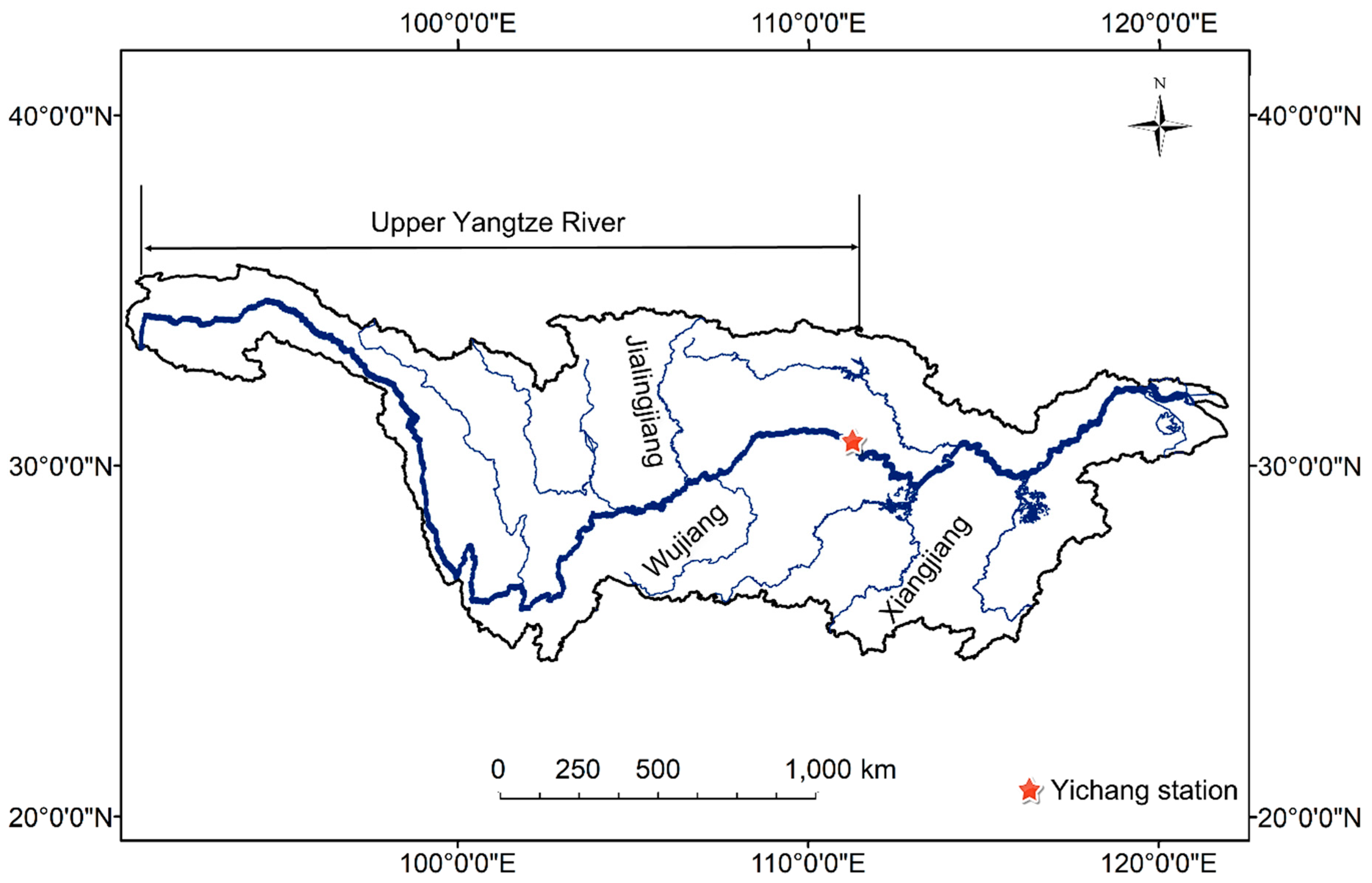
The Yangtze River, 6300 km long, originates from the Tibetan Plateau and ends in the Chongming Island in Shanghai (shown in Figure 1). The minimum annual rainfall of this basin is about 270 mm in the west and the maximum is about 1900 mm in the Southeast [17]. Because of the monsoon climate, more than 70% of its annual precipitation occurs in summer. The Yangtze River basin is prone to huge flood events and it has caused great damages to social prosperity and loss of life, and the flood in 1998 led to an economic loss of more than $20 billion [18]. To this end, many measures have been taken in recent years. The Three Gorges Project was built in the Yangtze River and it has been completed in 2003, the main function of which is flood control. Besides, the streamflow is also sensitive to climate changes [19], which makes it more necessary and important to reassess the flood conditions and forecast future risks in this region.

According to its geographical and climatic characteristics, the Yangtze River is subdivided into three sections, where Yichang is the dividing point between the upper and middle reaches. The Yichang station, located 44 km downstream of the Three Gorges Reservoir, is an important monitoring station for hydrological regimes in the upper Yangtze River. In this study, daily averaged streamflow records at the Yichang station from 1949 to 2012 were collected for research, and the flood peak and 7-day flood volume series were extracted from the data using the block maximum approach. The flood peak (P), is defined as the discharge of the annual maximum flood; the 7-day flood volume (V), is defined as the integral of the annual maximum 7-day flood and time, it does not necessarily include the day of the annual maximum flood. There are no missing values in the records for this period.

3. Methodology

3.1. Trend Analysis

3.1.1. Univariate Trend Test

The Mann-Kendall (M-K) trend test [20,21] is a rank-based method which is widely adopted in hydro-meteorological studies for detecting the trend in a time series. For a hydrological variable x with n years of records, the test is based on the statistic value S defined by the following formula:

$$S={\displaystyle \sum _{1\le i<j\le n}\mathrm{sgn}(x_j-x_i),\mathrm{sgn}(x_j-x_i)=\{\begin{array}{l}+1\mathrm{if}(x_j-x_i)>0\\ 0\hspace{1em}\mathrm{if}(x_j-x_i)=0\\ -1\mathrm{if}(x_j-x_i)<0\end{array}}$$

(1)

Under a null hypothesis of no trend, the statistical S is approximately normally distributed with zero mean and its variance:

$$Var\left(S\right)=\left[n\left(n-1\right)\left(2n+5\right)\right]/18$$

(2)

The flood peak and volume series were examined with a two-sided test given a 0.05 significance level in this study.

3.1.2. Multivariate Trend Test

The Covariance Sum Test (CST), introduced by Hirsch and Slack [22], was adopted as an extension of the univariate M-K test for detecting trends in multivariate correlated data in this study. In multivariate cases, the univariate statistic S^(u) (u = 1, 2,…, d) for each component of the variables is calculated first. S = (S⁽¹⁾, S⁽²⁾,…, S^(d)) is a d-dimensional vector with a covariance matrix C_M = (c_u,v)_{u,v=1,……d}, in which c_u,v = cov(M^(u),M^(v)). The covariate terms are calculated with the following equations [23]:

$${\widehat{c}}_{u,v}=\frac{t_{u,v}+r_{u,v}}{3}foru\ne v$$

(3)

where

$$t_{u,v}={\displaystyle \sum _{i\le i<j\le n}\mathrm{sgn}(x_j^{(u)}-x_i^{(u)})(}{x}_j^{(v)}-x_i^{(v)})$$

(4)

$$r_{u,v}={\displaystyle \sum _{i,j,k=1}^n\mathrm{sgn}(x_k^{(u)}-x_j^{(u)})(x_k^{(v)}-x_i^{(v)})}$$

(5)

The multivariate M-K test is based on the statistic S_m, given as:

$$S_m={\displaystyle \sum _{u=1}^d{S}^{(u)}}$$

(6)

Under a null hypothesis, the statistic S_m is asymptotically normal with zero mean and its variance is given as:

$$Var(S_m)={\displaystyle \sum _{u=1}^{d}Var(S^{(u)})+2{\displaystyle \sum _{v=1,u=1}^{d,v-1}{c}_{u,v}}}$$

(7)

For a given significance level, the application of the CST is similar to that of the univariate M-K test.

3.2. Time Varying Copula

Under a changing environment, both the marginal distribution of hydrological variables and the dependence structure between them might be changing and the non-stationary copula is a perfect solution to this problem. In bivariate cases, based on the conventional copula theory, the time varying copula is defined as follows [14]:

$$H_{Y_1,Y_2}(y_1,y_2)=C\left[F_1\left(y_1|{\theta }_1^t\right),F_2\left(y_2|{\theta }_2^t\right)|{\theta }_c^t\right]$$

(8)

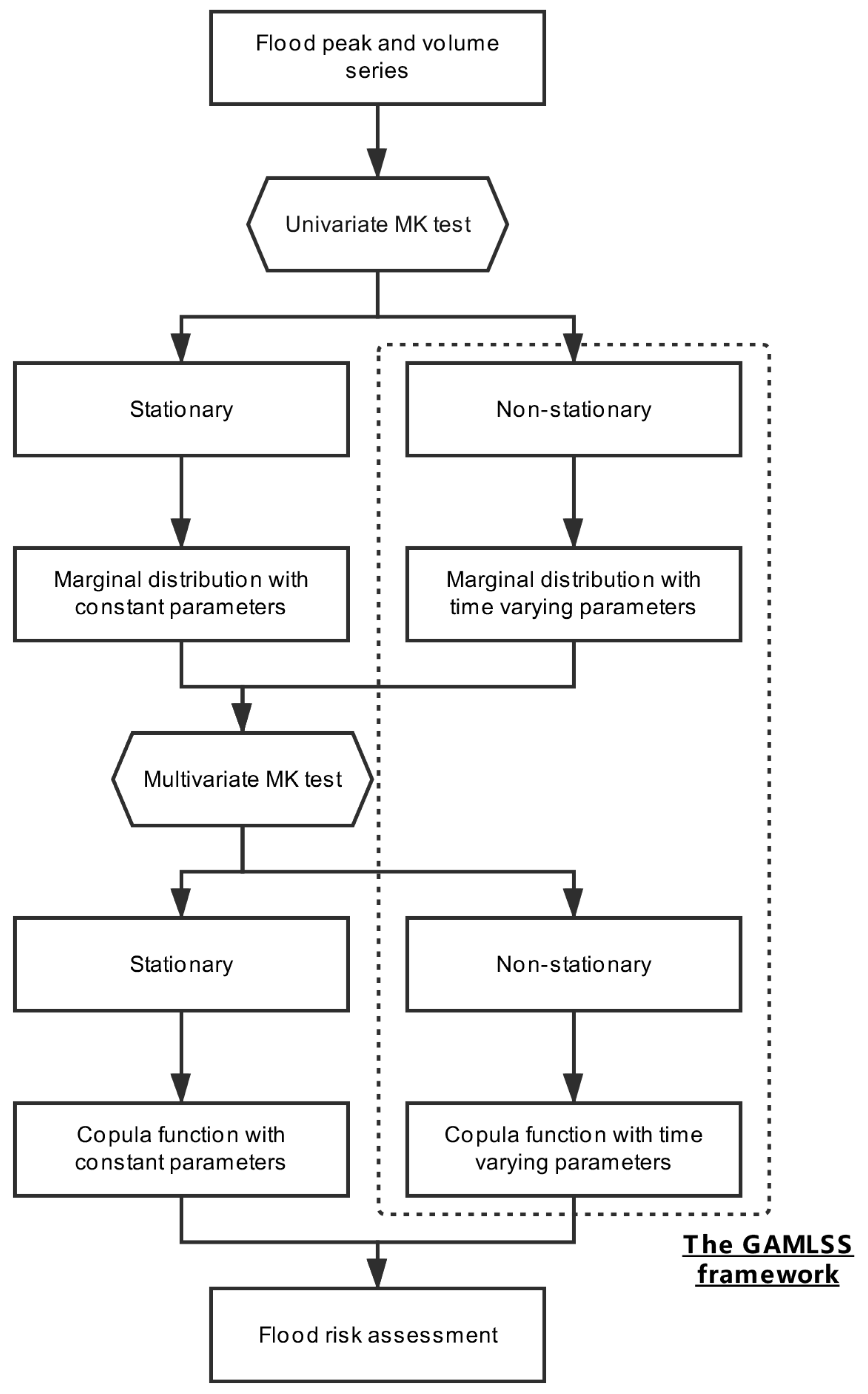
where F₁( ) and F₂( ) are marginal distributions for the variables Y₁ and Y₂, C( ) is the copula function; ${\theta }_1^t$ and ${\theta }_2^t$ are parameters for the marginal distributions, and ${\theta }_c^t$ is the parameter for the copula function, and the superscript t means the parameters are time varying. The procedure for how to construct a time varying copula model is presented in Figure 2.

3.2.1. Marginal Distribution

To investigate the flood characteristics, various probability distributions have been recommended and studied in flood modeling researches [24]. Six widely used distributions, including Gamma, Weibull, Gumbel, Logistic, Lognormal and Pearson type III distributions, were selected as candidates in this study for flood peak and 7-day flood volume series. Parameters of the distributions were estimated by the Generalized Additive Models in Location, Scale and Shape (GAMLSS) [25], which has been widely used in non-stationary modeling recently [26,27]. In a GAMLSS framework, the observation of a variable y is assumed to follow a distribution with a probability density function (PDF) f (y|θ), and the parameter vector θ^T is described as a function of explanatory variables and random effects. In case there are no additive terms, the distribution parameters can be denoted by a monotonic link function g_k( ) as:

$$g_k\left({\theta }_k\right)=X_k{\beta }_k={\beta }_{0k}+{\beta }_{1k}X+\cdots +{\beta }_{qk}{X}^q,k=1,2,\dots ,p$$

(9)

where X_k denote the explanatory variables, β_k are polynomial coefficients, p is the number of parameters, q is the degree of the polynomial, and q = 1 in this study to avoid over-parameterization. The location and scale parameters were related to the time covariate, including either one of them is time varying or both of them as time varying, and the shape parameter was treated as a constant. The stationary model was obtained by assuming that the parameters are independent of the explanatory variables. The optimal distribution was determined by the Akaike Information Criterion (AIC) [28] and the goodness-of-fit test was performed by the worm plot [29]. PDFs of the marginal distributions and their link functions are listed in

Table 1. Probability density functions of the marginal distributions and their link functions.

Distribution	Probability Density Function, f(x)	Link Function
		g(μ)	g(σ)
Gamma	$f(x)=\frac{1}{{({\sigma }^2\mu )}^{1/{\sigma }^2}}\frac{x^{\frac{1}{{\sigma }^2}-1}{e}^{-x/({\sigma }^2\mu )}}{\mathsf{\Gamma }(1/{\sigma }^2)}$	ln(μ)	ln(σ)
Weibull	$f(x)=\frac{\sigma x^{\sigma -1}}{{\mu }^{\sigma }}\exp {(-\frac{x}{\mu })}^{\sigma }$	ln(μ)	ln(σ)
Gumbel	$f(x)=\frac{1}{\sigma }\exp [\left(\frac{x-\mu }{\sigma }\right)-\exp (\frac{x-\mu }{\sigma })]$	μ	ln(σ)
Logistic	$f(x)=\frac{1}{\sigma }\left\{\exp \left[-\frac{x-\mu }{\sigma }\right]\right\}{\left\{1+\exp \left[-\left(\frac{x-\mu }{\sigma }\right)\right]\right\}}^{-2}$	μ	ln(σ)
Lognormal	$f(x)=\frac{1}{\sqrt{2\pi {\sigma }^2}}\frac{1}{x}\exp \left\{-\frac{{\left[\log (x)-\mu \right]}^2}{2{\sigma }^2}\right\}$	μ	ln(σ)
Pearson III	$f(x)=\frac{2}{\mu \sigma \epsilon \mathsf{\Gamma }(4/{\epsilon }^2)}{\left[\frac{2\left(x-\mu \right)}{\mu \sigma \epsilon }+\frac{4}{{\epsilon }^2}\right]}^{\frac{4}{{\epsilon }^2}-1}\exp \left[-\left(\frac{2\left(x-\mu \right)}{\mu \sigma \epsilon }+\frac{4}{{\epsilon }^2}\right)\right]$	ln(μ)	ln(σ)

Note: μ is the location parameter, σ is the scale parameter and ε is the shape parameter.

.

3.2.2. Copula Function

Among all copula families, the Archimedean copula is the most commonly used in hydrological modeling for its simple structure and good applicability [30]. In this study, four Archimedean copulas, namely the Clayton, Gumbel–Hougaard (GH), Frank, and Joe copulas, were adopted for the bivariate modeling of flood peak and volume series.

Similar to the marginal distributions, the parameter θ of the copula is linked to the time covariate as follows:

$$g_c(\theta )={\beta }_0+{\beta }_{1}t$$

(10)

where β₀ and β₁ are polynomial coefficients and t is the time. A brief description of these copulas and their link functions are presented in

Table 2. The description of the Archimedean copulas and their link functions.

Copula	C(u,v)	Range of θ	g(θ)
Clayton	$max({[u^{-\theta }+v^{-\theta }-1]}^{-\frac{1}{\theta }},0)$	θ > 0	ln(θ)
GH	$\exp \{-{[{(-\ln u)}^{\theta }+{(-\ln v)}^{\theta }]}^{1/\theta }\}$	θ ≥ 1	ln(θ)
Frank	$-\frac{1}{\theta }\ln [1+\frac{(e^{-\theta u}-1)(e^{-\theta v}-1)}{e^{-\theta }-1}]$	θ ≠ 0	ln(θ)
Joe	$1-{[{(1-u)}^{\theta }+{(1-v)}^{\theta }-{(1-u)}^{\theta }{(1-v)}^{\theta }]}^{1/\theta }$	θ ≥ 1	ln(θ)

.

Generally, there are three combinations of marginal distributions and copula functions for a time varying copula model, and the final model is determined according to the trend test results. The temporal variations among different copula models are captured by comparing the AIC values and the stationary model is taken as a benchmark. The Inference Function for Margins (IFM) method [31] was applied for the estimation of parameters.

3.3. Return Period, Risk of Failure and Reliability

3.3.1. Non-Stationary Return Period

The return period is essential in flood frequency analysis and usually used in risk quantification and evaluation [32]. In general, there are two interpretations of the return period, one of which is the expected waiting time (EWT) until the first event occurs. For a known design flood event (x = 0), X is defined as the waiting time until the event reoccurs for the first time, then the probability for X = x can be expressed using the following Equation [10]:

$$P(X=x)=(1-P_1)(1-P_2)(1-P_3)\dots (1-P_{x-1})P_x=P_x{\displaystyle \prod _{i=1}^{x-1}(1-P_i)},x=1,2,\dots ,\infty$$

(11)

where P_i is the exceeding probability of a design event for each year. The EWT return period T of the design event can thus be expressed as:

$$T=E(X)={\displaystyle \sum _{x=1}^{\infty }x{P}_x{\displaystyle \prod _{i=1}^{x-1}(1-P_i)}}=1+{\displaystyle \sum _{x=1}^{\infty }{\displaystyle \prod _{i=1}^x(1-P_i)}}$$

(12)

Another interpretation of the return period is that the expected number of events (ENE) in T years is one [33]. For a period of T years, N is the number of the design event, the expected value of which is calculated by:

$$E(N)={\displaystyle \sum _{i=1}^{T}E(I(P_i))=}{\displaystyle \sum _{i=1}^T{P}_i}$$

(13)

where I is an indicator variable. The ENE return period T is obtained when the solution to Equation (13) is equal to 1, as follows:

$$1={\displaystyle \sum _{i=1}^T{P}_i}$$

(14)

In terms of bivariate frequency analysis, the design event is always divided into two cases, namely case AND (Y₁ ≥ y₁ and Y₂ ≥ y₂) and case OR (Y₁ ≥ y₁ or Y₂ ≥ y₂), which can be defined by two exceeding probabilities using copula theory as follows:

$$P（Y_1\ge y_{1}and{Y}_2\ge y_2）=1-F_1(y_1)-F_2(y_2)+C(F_1(y_1),F_2(y_2)),$$

(15)

$$P(Y_1\ge y_{1}or{Y}_2\ge y_2)=1-C(F_1(y_1),F_2(y_2))$$

(16)

Under the stationary assumption, the exceeding probabilities P_i for each year are exactly the same so that both the two interpretations lead to the same result, T = 1/P_i, which can be divided into two cases, specifically, using the following equations [34]:

$$T^{AND}=\frac{1}{P(Y_1\ge y_{1}and{Y}_2\ge y_2)}=\frac{1}{1-F_1(y_1)-F_2(y_2)+C(F_1(y_1),F_2(y_2))}$$

(17)

$$T^{OR}=\frac{1}{P(Y_1\ge y_{1}or{Y}_2\ge y_2)}=\frac{1}{1-C(F_1(y_1),F_2(y_2))}$$

(18)

It is obvious that the stationary return period defined in Equations (17) and (18) do not provide more information than only the exceeding probabilities. Under non-stationary assumptions, since the exceeding probabilities for each year are different, Equations (17) and (18) are no longer valid, and the EWT and ENE definitions can lead to different return periods. However, the definition of EWT includes calculation of the exceeding probabilities for an infinite period, which is hard to predict and has a risk of not converging. Besides, the rate of convergence of EWT may be influenced by the selected distribution to some extent [13]. Thus, the EWT definition is not taken for comparison in this study.

3.3.2. Risk of Failure and Reliability

The risk of failure, defined as the probability that a critical event occurs at least once in its design life, has become increasingly popular in non-stationary risk analysis. It provides a different perspective for evaluating flood risks from the return period. For n years of design life, the probability R that at least a failure was observed with exceeding probabilities P_i in the ith year is given as:

$$R=1-{\displaystyle \prod _{i=1}^n(1-P_i)}$$

(19)

where P_i can be either P_AND or P_OR given above in bivariate cases. Correspondingly, the reliability, r, is defined as the probability that no design flood event will happen in the next n years, given as:

$$r=1-R={\displaystyle \prod _{i=1}^n(1-P_i)}$$

(20)

4. Results

4.1. The Trend Test

The flood peak P and volume V series were extracted from the data and examined first. Given α = 0.05, the threshold values for significant trends are ±1.96. According to the univariate M-K test, the statistic result for the flood peak is −2.06 and it is −2.05 for the flood volume, indicating a significant decreasing trend for both of the two series. Moreover, according to the multivariate M-K test, the statistic result is −2.40, indicating a significant bivariate decreasing trend for the two variables. The results demonstrated that the stationary assumption may no longer be valid for the streamflow series at the Yichang station—not only the time varying marginal distributions, but also a time varying copula is needed in the flood frequency analysis in this region. Thus, we have two models for research in the subsequent sections, which are: Model 1, the stationary model with constant parameters; and model 2, the non-stationary model with both the marginal distribution and copula function parameters varying with time.

4.2. Marginal Distribution

The six distributions were tested to fit the marginal distributions of the flood peak and volume series, and the best-fitted one was selected according to minimum AIC values. For the flood peak series, the Weibull was the best-fitted distribution under the stationary assumption and the Gamma was the best-fitted distribution under the non-stationary assumption. A decreasing trend was detected in the location parameter while the scale parameter showed an increasing trend. On the other hand, the Logistic distribution was the most appropriate distribution for the flood volume series under both stationary and non-stationary assumptions, and a decreasing trend was detected in the location parameter while the scale parameter is constant. The optimal distributions and their parameters are presented in

Table 3. The optimal marginal distributions and their parameters.

Series	Type	Distribution	μ	σ	AIC
P (m3/s)	Stationary	Weibull	53,585.83	6.74	1341.9
	Non-stationary	Gamma	exp(10.90 − 0.0026t)	exp(−2.20 + 0.0116t)	1339.9
V (106 m3)	Stationary	Logistic	26,542.00	2444.02	1258.4
	Non-stationary	Logistic	28,239.69 − 53.43t	2387.50	1256.6

. The time varying distributions perform better than the stationary ones according to AIC values. The worm plots for time varying marginal distributions were presented in Figure 3. All points are within the 95% confidence interval and the selected distributions have enough fitting quality.

4.3. Copula Modeling

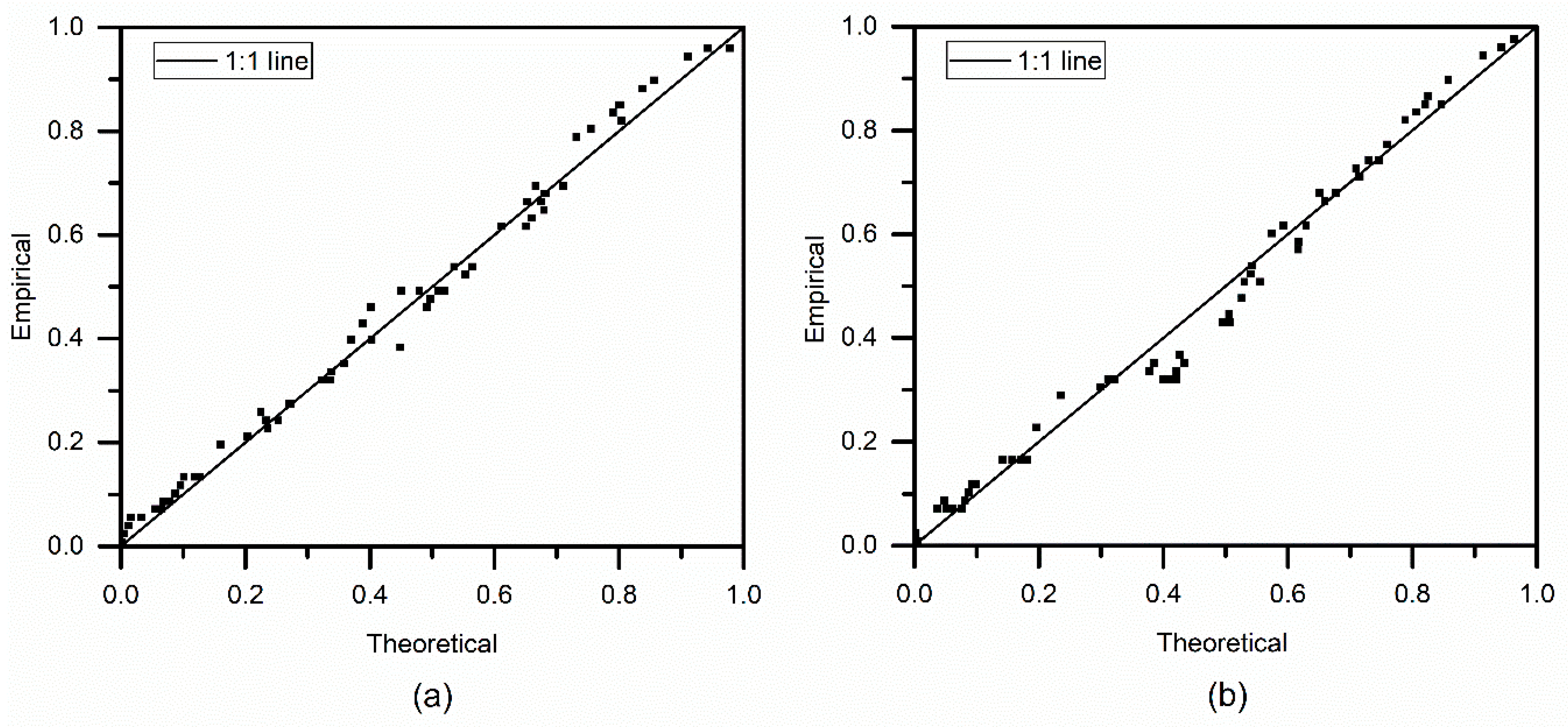
The dependence structure between flood peak and volume series was explored first in the multivariate frequency analysis. Using the three widely used relationship coefficients, the Pearson’s ρ is 0.90, Kendall’s tau is 0.75, and the Spearman’s rho is 0.91, indicating that the two variables are strongly correlated.

Table 4. The parameters and goodness-of-fit tests for candidate copulas.

Model	Copula Function	θ	AIC
1	Clayton	3.70	−94.31
	GH	3.06	−87.33
	Frank	12.88	−101.80
	Joe	3.43	−63.52
2	Clayton	exp(−0.0064t + 1.24)	−76.98
	GH	exp(−0.0048t + 1.34)	−98.05
	Frank	exp(−0.0039t + 2.69)	−102.36
	Joe	exp(−0.0052t + 1.55)	−77.45

summarizes the parameters and goodness-of-fit results for the two models, and it can be found that all the copula functions of model 2 detected a decreasing trend of θ, which means the correlation relationship between the two variables weakened over time. Almost all the AIC values of non-stationary models are smaller than the stationary model when using the same copula function, except for the Clayton copula. The Frank copula of model 2 is the best fit for bivariate modeling of flood peak and volume among all scenarios. The relationship between empirical and theoretical probabilities for the Frank copula under stationary and non-stationary conditions was plotted in Figure 4. All points are located near the 1:1 line, indicating satisfactory fitting performance.

4.4. Flood Risk Assessment

4.4.1. The Non-Stationary Return Period

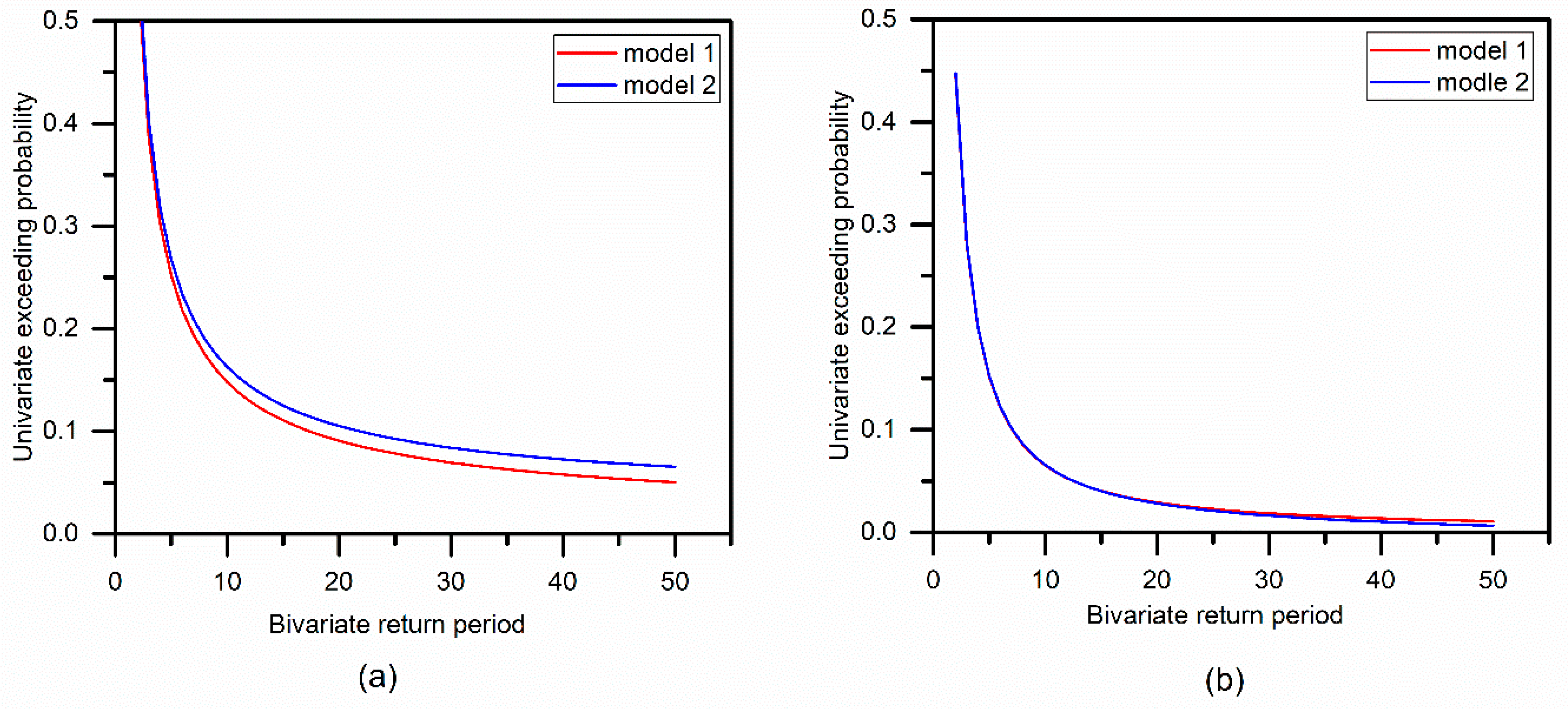
Based on the selected copula and estimated parameters for each model, the bivariate non-stationary return periods can be estimated by substituting Equations (15) and (16) to Equation (14). It should be noted that the non-stationary return period was defined for each year rather than the whole series. Following the Chinese flood guidelines [35], the unique combination of design flood peak and volume is determined by setting them to be of the same univariate frequency, which was a uniform procedure for similar calculations of design values in past studies [36]. Specifically, for the year 2012, the univariate exceeding probability against the bivariate non-stationary return period was presented in Figure 5. In case AND from Figure 5a, for a given return period, the univariate exceeding probability of model 2 is bigger than that of model 1, implying that the non-stationary model is safer than the stationary model under the same design standard. On the other hand, the non-stationarities have a very small influence on the return period of case OR, as shown in Figure 5b. The result was further evaluated by the design values. For example, the univariate exceeding probabilities under 10 years of the bivariate return period in case OR are both 0.065 for the two models, while the designed flood peaks (m³/s) are 62,202 and 63,127, respectively, and the designed flood volumes (10⁶ m³/s) are 33,054 and 31,165, respectively. Model 2 is characterized by a higher flood peak and lower flood volume compared with model 1, which may be attributed to the time varying marginal distributions.

4.4.2. Risk of Failure and Reliability

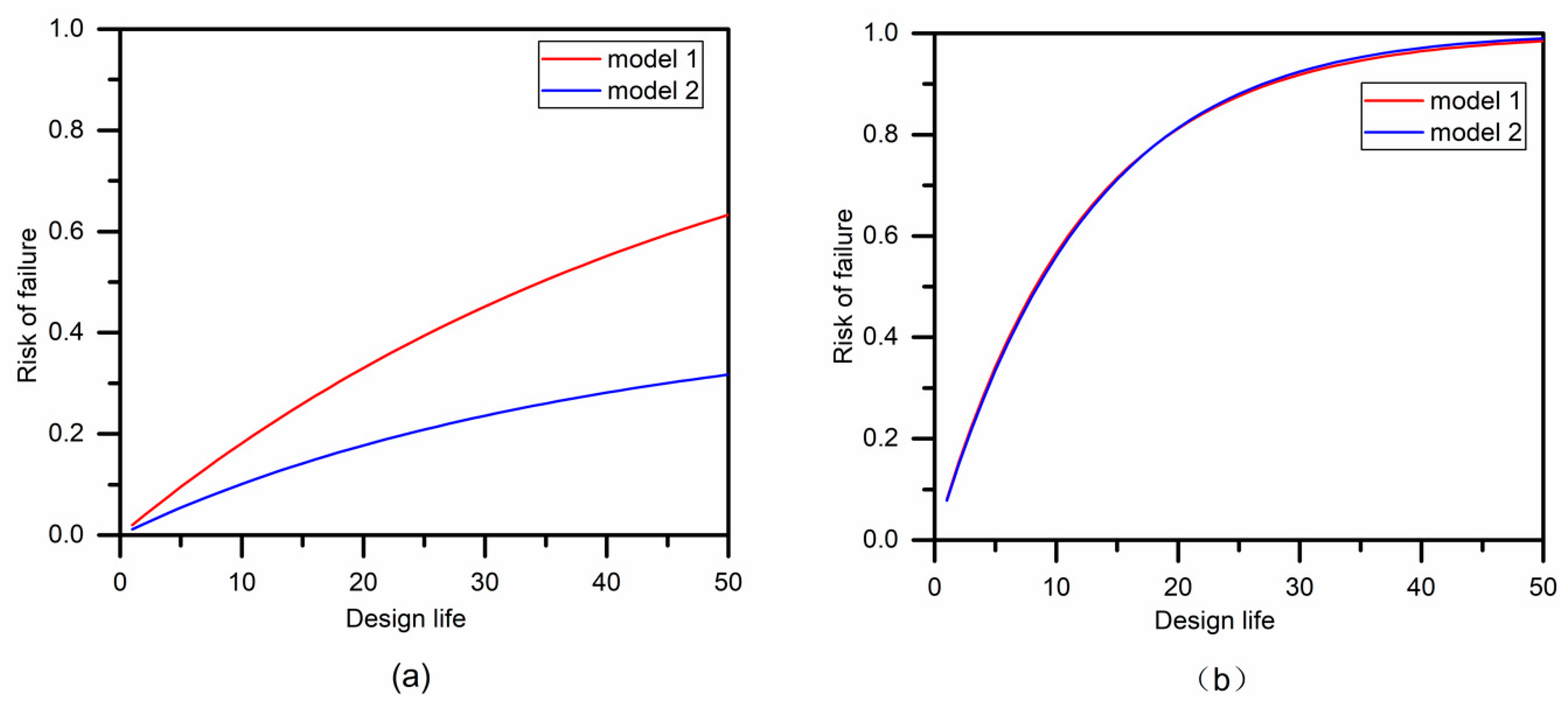
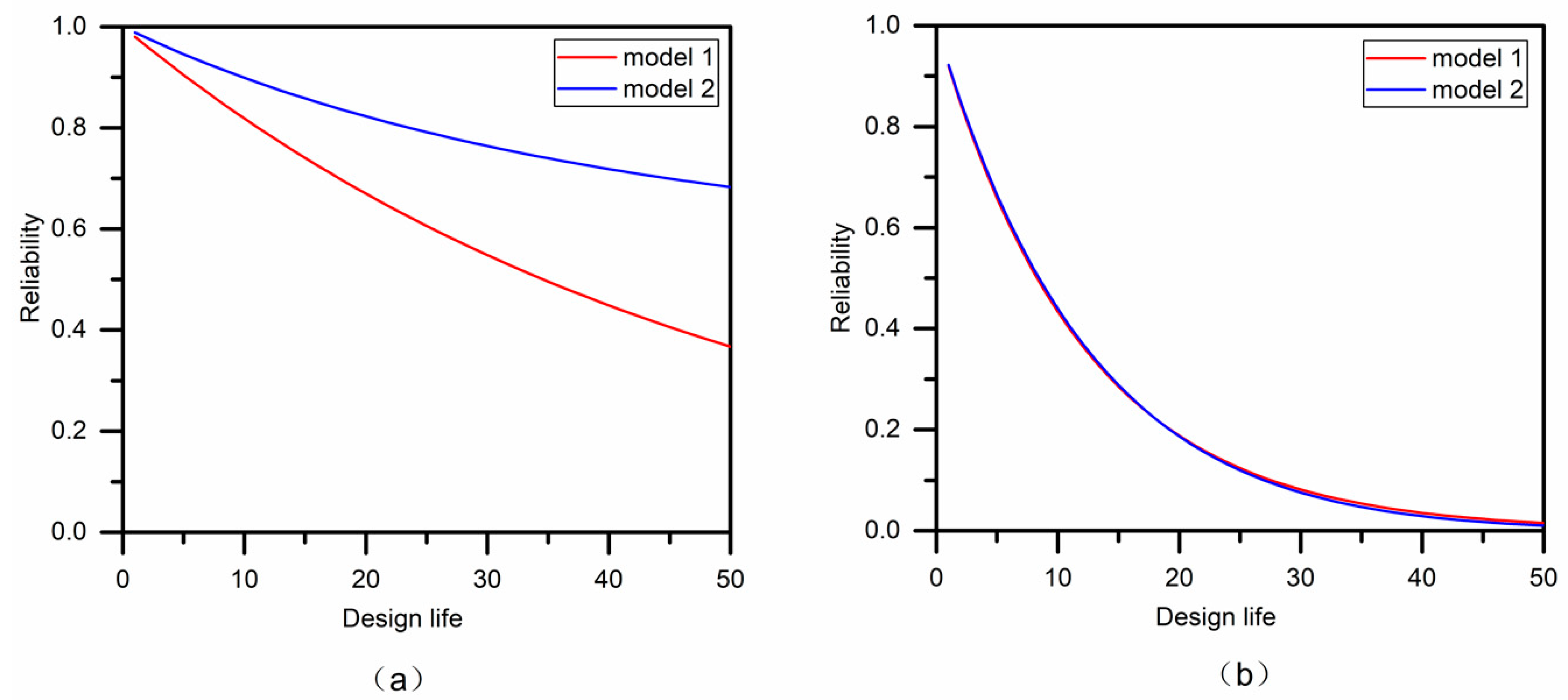
Given the initial flood peak (63,059 m³/s) and volume (33,738 × 10⁶ m³/s) with 20 years of univariate return period under the stationary assumption, the risk of failure of the design flood events for model 1 and model 2 in the next 50 years are calculated and plotted in Figure 6. Figure 6a shows the risk of failure for case AND. Under the stationary assumption, the risk of failure R increased rapidly with the design life n, as shown by the red line. However, due to non-stationarities, the flood risk is smaller than the stationary model, and the rate of growth decreased as presented by the blue line. On the other hand, Figure 6b shows the risk of failure for case OR, the conclusions of which are completely different from that of case AND. In total, the R values of case OR are nearly the same between model 1 and model 2, indicating that the non-stationary properties have a very small influence on the risk of failure for the flood event case OR. Figure 7 presents the results of reliability for the two models, which are similar to those of Figure 6. The results suggested that the hydrologic facilities controlled by design flood event case OR are more stable under the changing environment in the study region, but the risks are much bigger than that of case AND.

5. Discussion

The multivariate analysis is more complicated than the univariate analysis in terms of different combinations of hydrological variables and various design events. In past literature on time varying copulas, the assessment of dynamic risks is a difficult task. Jiang et al. [14] used the joint return period for bivariate non-stationary modeling of low flows in the Hanjiang River, but the definition is similar to that under the stationary assumption. Zhang et al. [37] abandoned the return period and used the exceeding probabilities instead for non-stationary flood frequency analysis in the Wangkuai Reservoir catchment. The bivariate non-stationary return period and risk of failure used in this study provided an explicit measure of risk with a robust theoretical basis, thus filling up the current knowledge gap. The performances of case AND and case OR can be completely different in this study, and more attention can be paid to different kinds of return periods for multivariate flood events, such as Kendall’s return period, the structure-based return period, and so on. However, we should also keep in mind that T^AND and T^OR and any other kind of return period are only different descriptions of the underlying mechanisms of design structures and must be used accordingly. It is important to figure out what type of event is used in the practical application and how to evaluate the effect of non-stationarity on flood risk under this specific condition.

6. Conclusions

In summary, this paper built a non-stationary copula model for bivariate flood frequency analysis in the Yangtze River basin, where the streamflow records from 1949 to 2012 at the Yichang station were used as a practical application. Flood peak is defined as the annual maximum flooding, while 7-day flood volume is the integral of annual maximum 7-day flood and time. The non-stationary return period and risk of failure were evaluated for flood risk assessment. The main conclusions are listed as follows.

(1)

Both univariate and multivariate M-K trend tests were used to examine the temporal variations between flood characteristics, and the results revealed severe non-stationary properties, indicating that the stationary assumption is invalid, and a non-stationary copula model is needed for hydrological modeling in this region.

(2)

The flood peak and volume series were fitted by 6 marginal distributions under stationary and non-stationary situations, and the appropriate distributions vary correspondingly. The Weibull and Logistic distributions were selected for flood peak and volume under the stationary assumption, while the Gamma and Logistic distributions were selected under the non-stationary assumption. The flood peak and volume series presented decreasing trends in their location parameters. Four copula functions were applied to investigate the dependence structure between flood variables, and the Frank copula was selected as the most appropriate. The non-stationary model performs better than the copula with constant parameters according to AIC values. The copula parameters of the non-stationary model detected a decreasing trend, which means the dependence structure between flood variables also weakened over time.

(3)

The joint non-stationary return period was calculated for comparison, and the results varied with different design flood events. Compared with the stationary model, in case AND, the flood risk of non-stationary models decreased as a result of the decreased parameters of both marginal distributions and copula functions. While in case OR, the effect of the non-stationary properties is almost negligible. As for the design values, the non-stationary model is characterized by a higher flood peak and lower flood volume. The bivariate risk of failure of 50 years of design life was also estimated, and the conclusions were similar to those obtained by the return period. The effect of non-stationarity is more inclined to case AND rather than case OR, and the non-stationary model is safer than the stationary model in case AND.

The streamflow series at the Yichang station showed significant non-stationary properties according to our research, and the non-stationary copula model can better describe the temporal variations. The bivariate non-stationary return period and risk of failure may throw light on the extension of conventional concepts and serve as valuable tools for flood risk assessment in a changing environment. Time was used as a covariate in this study for both the marginal distribution and copula function. However, it is not recommended in non-stationary modeling because of its lack of physical meanings. Moreover, the time varying trend obtained through past data may not be consistent after 50 or 100 years, and the reliability of predicted results needs to be carefully considered. Some physical-based variables, such as the climate index, can be taken into account in future studies.

References

- Selenica, A.; Kuriqi, A.; Ardicioglu, M. Risk assessment from floodings in the rivers of albania. In Proceedings of the International Balkans Conference on Challenges of Civil Engineering, Tirana, Albania, 23–25 May 2013. [Google Scholar]
- Kuriqi, A.; Ardiçlioǧlu, M. Investigation of hydraulic regime at middle part of the loire river in context of floods and low flow events. Pollack Period. 2018, 13, 145–156. [Google Scholar] [CrossRef]
- Deng, X.; Ren, W.; Feng, P. Design flood recalculation under land surface change. Nat. Hazards 2016, 80, 1153–1169. [Google Scholar] [CrossRef]
- Oliver, J.; Qin, X.S.; Larsen, O.; Meadows, M.; Fielding, M. Probabilistic flood risk analysis considering morphological dynamics and dike failure. Nat. Hazards 2018, 91, 287–307. [Google Scholar] [CrossRef]
- Milly, P.C.D.; Betancourt, J.; Falkenmark, M.; Hirsch, R.M.; Kundzewicz, Z.W.; Lettenmaier, D.P.; Stouffer, R.J. Stationarity is dead: Whither water management? Science 2008, 319, 573–574. [Google Scholar] [CrossRef] [PubMed]
- Zhang, Q.; Zhou, Y.; Singh, V.P.; Chen, X. The influence of dam and lakes on the yangtze river streamflow: Long-range correlation and complexity analyses. Hydrol. Process. 2012, 26, 436–444. [Google Scholar] [CrossRef]
- Ishak, E.H.; Rahman, A.; Westra, S.; Sharma, A.; Kuczera, G. Evaluating the non-stationarity of australian annual maximum flood. J. Hydrol. 2013, 494, 134–145. [Google Scholar] [CrossRef]
- O’Brien, N.L.; Burn, D.H. A nonstationary index-flood technique for estimating extreme quantiles for annual maximum streamflow. J. Hydrol. 2014, 519, 2040–2048. [Google Scholar] [CrossRef]
- Li, J.; Tan, S. Nonstationary flood frequency analysis for annual flood peak series, adopting climate indices and check dam index as covariates. Water Resour. Manag. 2015, 29, 5533–5550. [Google Scholar] [CrossRef]
- Salas, J.D.; Obeysekera, J. Revisiting the concepts of return period and risk for nonstationary hydrologic extreme events. J. Hydrol. Eng. 2014, 19, 554–568. [Google Scholar] [CrossRef]
- Serinaldi, F. Dismissing return periods! Stoch. Environ. Res. Risk Assess. 2014, 29, 1179–1189. [Google Scholar] [CrossRef] [Green Version]
- Du, T.; Xiong, L.; Xu, C.-Y.; Gippel, C.J.; Guo, S.; Liu, P. Return period and risk analysis of nonstationary low-flow series under climate change. J. Hydrol. 2015, 527, 234–250. [Google Scholar] [CrossRef]
- Yan, L.; Xiong, L.; Guo, S.; Xu, C.-Y.; Xia, J.; Du, T. Comparison of four nonstationary hydrologic design methods for changing environment. J. Hydrol. 2017, 551, 132–150. [Google Scholar] [CrossRef]
- Jiang, C.; Xiong, L.; Xu, C.Y.; Guo, S. Bivariate frequency analysis of nonstationary low-flow series based on the time-varying copula. Hydrol. Process. 2015, 29, 1521–1534. [Google Scholar] [CrossRef]
- Ahn, K.H.; Palmer, R.N. Use of a nonstationary copula to predict future bivariate low flow frequency in the connecticut river basin. Hydrol. Process. 2016, 30, 3518–3532. [Google Scholar] [CrossRef]
- Sarhadi, A.; Burn, D.H.; Ausín, M.C.; Wiper, M.P. Time varying nonstationary multivariate risk analysis using a dynamic bayesian copula. Water Resour. Res. 2016, 52. [Google Scholar] [CrossRef]
- Yu, F.; Chen, Z.; Ren, X.; Yang, G. Analysis of historical floods on the yangtze river, china: Characteristics and explanations. Geomorphology 2009, 113, 210–216. [Google Scholar] [CrossRef]
- Chen, L.; Singh, V.P.; Shenglian, G.; Hao, Z.; Li, T. Flood coincidence risk analysis using multivariate copula functions. J. Hydrol. Eng. 2012, 17, 742–755. [Google Scholar] [CrossRef]
- Su, B.; Huang, J.; Zeng, X.; Gao, C.; Jiang, T. Impacts of climate change on streamflow in the upper yangtze river basin. Clim. Chang. 2017, 141, 533–546. [Google Scholar] [CrossRef]
- Mann, H.B. Nonparametric tests against trend. Econometrica 1945, 13, 245–259. [Google Scholar] [CrossRef]
- Kendall, M.G. Rank Correlation Measures; Charles Griffin: London, UK, 1975. [Google Scholar]
- Hirsch, R.M.; Slack, J.R. A nonparametric trend test for seasonal data with serial dependence. Water Resour. Res. 1984, 20, 727–732. [Google Scholar] [CrossRef]
- Chebana, F.; Ouarda, T.B.M.J.; Duong, T.C. Testing for multivariate trends in hydrologic frequency analysis. J. Hydrol. 2013, 486, 519–530. [Google Scholar] [CrossRef]
- Rizwan, M.; Guo, S.; Xiong, F.; Yin, J. Evaluation of various probability distributions for deriving design flood featuring right-tail events in pakistan. Water 2018, 10, 1603. [Google Scholar] [CrossRef]
- Rigby, R.A.; Stasinopoulos, D.M. Generalized additive models for location, scale and shape. J. R. Stat. Soc. Ser. C-Appl. Stat. 2005, 54, 507–544. [Google Scholar] [CrossRef]
- Yan, L.; Xiong, L.; Liu, D.; Hu, T.; Xu, C.-Y. Frequency analysis of nonstationary annual maximum flood series using the time-varying two-component mixture distributions. Hydrol. Process. 2017, 31, 69–89. [Google Scholar] [CrossRef]
- Zhang, D.-D.; Yan, D.-H.; Wang, Y.-C.; Lu, F.; Liu, S.-H. Gamlss-based nonstationary modeling of extreme precipitation in Beijing–Tianjin–Hebei region of china. Nat. Hazards 2015, 77, 1037–1053. [Google Scholar] [CrossRef]
- Akaike, H. A new look at the statistical model identification. IEEE Trans. Autom. Control 1974, 19, 716–723. [Google Scholar] [CrossRef]
- Buuren, S.; Van Fredriks, M. Worm plot: A simple diagnostic device for modelling growth reference curves. Stat. Med. 2010, 20, 1259–1277. [Google Scholar] [CrossRef] [PubMed]
- Kang, L.; Jiang, S. Bivariate frequency analysis of hydrological drought using a nonstationary standardized streamflow index in the Yangtze river. J. Hydrol. Eng. 2019, 24, 05018031. [Google Scholar] [CrossRef]
- Joe, H. Multivariate Models and Multivariate Dependence Concepts; Chapman and Hall/CRC: New York, NY, USA, 1997. [Google Scholar]
- Zhang, Q.; Gu, X.; Singh, V.P.; Xiao, M.; Chen, X. Evaluation of flood frequency under non-stationarity resulting from climate indices and reservoir indices in the east river basin, china. J. Hydrol. 2015, 527, 565–575. [Google Scholar] [CrossRef]
- Cooley, D. Return periods and return levels under climate change. In Extremes in a Changing Climate; Springer: Dordrecht, The Netherlands, 2013; pp. 97–114. [Google Scholar]
- Salvadori, G.; De Michele, C.; Kottegoda, N.T.; Rosso, R. Extremes in Nature: An. Approach using Copulas; Springer Science & Business Media: Dordrecht, The Netherlands, 2007; Volume 56. [Google Scholar]
- Ministry of Water Resources. Regulation for Calculating Design Flood of Water Resources and Hydropower Projects; China Water&Power Press: Beijing, China, 2006. [Google Scholar]
- Li, T.; Guo, S.; Chen, L.; Guo, J. Bivariate flood frequency analysis with historical information based on copula. J. Hydrol. Eng. 2012, 18, 1018–1030. [Google Scholar] [CrossRef]
- Zhang, T.; Wang, Y.; Wang, B.; Tan, S.; Feng, P. Nonstationary flood frequency analysis using univariate and bivariate time-varying models based on gamlss. Water 2018, 10, 819. [Google Scholar] [CrossRef]
Figure 1.
A map of the Yangtze River basin.
Figure 2.
The procedure for constructing the time varying copula model.
Figure 3.
Worm plots for the time varying marginal distribution of (a) the flood peak series and (b) the flood volume series.
Figure 4.
A comparison of empirical and theoretical probabilities for the Frank copula (a) under the stationary condition and (b) under non-stationary condition.
Figure 5.
The univariate exceeding probability against the non-stationary return period for (a) case AND and (b) case OR.
Figure 6.
Bivariate risk of failure as a function of design life for (a) case AND and (b) case OR.
Figure 7.
Reliability as a function of design life for (a) case AND, and (b) case OR.