Modeling of Hydrodynamics and Dilution in Coastal Waters


Department of Civil Engineering, Gazi University, 06570 Ankara, Turkey
Water 2019, 11(1), 83; https://doi.org/10.3390/w11010083
Submission received: 13 December 2018
/
Revised: 28 December 2018
/
Accepted: 30 December 2018
/
Published: 5 January 2019
(This article belongs to the Section Hydraulics and Hydrodynamics)
Abstract
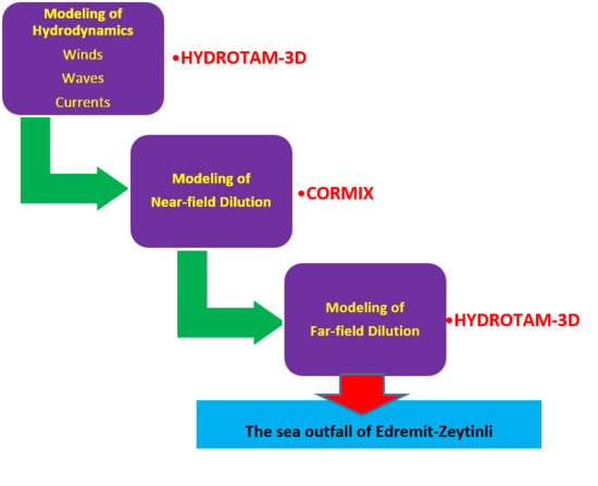
:Sea outfall systems are preferred to refinery systems because of the assimilation capacity of the sea as an economical choice. If sea outfall systems are chosen, the location of the sea outfall is critical for preventing the return of wastewater to the coastal zone and recovery back into an ecosystem. On the basis of the regulation of water pollution control, bacterial concentration needs to be below a certain value in the protected area. The primary effects on dilution are coastal currents generated by wind and transport of wastewater in closed or semi-closed coastal regions, as found in Turkey. Accurate predictions of wind and wave climates and currents are critical in sea outfall planning. In this study, the wind climate is determined from the data provided by the Edremit and Ayvalık Meteorological Stations and European Centre for Medium-Range Weather Forecasts operational archive at the coordinates of 39.50° N–26.90° E. Wind, wave, and current roses are prepared by HYDROTAM-3D. CORMIX was used for the near-field dilution, and HYDROTAM-3D, a three-dimensional hydrodynamic transport model, was used for the far-field dilution of the pollutant. The results of near-field and far-field dilution modeling show that the sea outfall of Edremit–Zeytinli meets the legal regulations.
1. Introduction
The coastal environment is used as a source of food and recreation as well as a final sink for wastes. There is an obvious potential conflict. With increasing industrialization and urbanization, urban and industrial community waste has increasingly been disposed of in coastal waters; this pollution brings habitat loss and degradation in marine ecosystems. The need for coastal pollution control has increased significantly. Disposal is by means of a pipeline on the seabed with a multiport diffuser. The effluent density determines the behavior of the pollutant jet. It can be positive or negative. When the effluent density is smaller than the density of ambient water, then it is called positively buoyant jet, oppositely it is called negatively buoyant jet or dense jet. As an example, thermal discharges from cooling water systems results positively buoyant jets. Salted discharges from desalination plants cause negatively buoyant jets [1,2,3]. The wastewater, having a density close to that of fresh water, rises to the surface and entrains the surrounding sea water and becomes diluted. If the ambient sea water is stratified, the diluted waste mixture may be trapped below the sea surface where its density is similar to that of the sea water (near-field dilution). However, if water is shallow, as in the case of the bulk of coastal waters, the diluted waste mixture, with a density less than the sea water, rises to the surface, and it is further diluted by the sea currents and turbulence (far-field dilution) [4]. The near-field mixing is a result of buoyancy and initial momentum. It is significant over distances of 10–1000 m and a duration of 1–10 min. The far-field mixing occurs because of the advection and diffusion by the coastal currents and turbulence. It is significant over distances of 100 m to 10 km and duration of 1–20 h [5]. During the actual dilution process, pathogens die away and become inactive. The quality of water near the coast is an outcome of the net result of any treatment, inactivation, and dilution of discharged waste [6]. To understand the complex and vital phenomena of the mixing process, numerical, analytical, physical models, and field experiments can be used [7,8,9,10]. The integration of this knowledge with different methodologies can deal with the complexity of hydrodynamic and hydraulic studies.
Empirical methods are appropriate for simple geometries and flows. A zero-equation turbulence closure can be assumed with a constant eddy viscosity. Solutions of empirical models are generally related to the final dilution values. Integral methods define jet-cross-sectional distribution functions a priori and use the conversion of the governing equations into ordinary differential equations. Dilutions and trajectories of the plume in an infinite water body are determined with integral methods. Numerical methods are needed for more complex geometries and flows. Advanced turbulence closure such as k-ɛ model, Reynolds-stress or Large Eddy simulation models is mandatory. The solutions of numerical methods are difficult, but they give complete results of dilutions and trajectories in limited water bodies [11].
Because of the complexity of turbulent transport mechanisms, different modeling techniques have been developed. Some examples of models are: length scale models based on dimensional analysis and experimental data [12], entrainment models based on nonlinear stratification and non-uniform velocities [13,14], computational fluid dynamic (CFD) models based on turbulence closure assumptions such as direct numerical simulation models, large eddy simulation models, and Reynolds-decomposition models [15,16]. Far-field circulation models are typically two- or three-dimensional (3D). Two-dimensional depth-averaged models are useful for unstratified shallow waters. In deeper waters, 3D models are needed, especially if wind shear effects, baroclinic processes, and density stratification exist [5,17,18,19].
The determination of the effects of a sanitary pollutant on the coastal area is necessary to plan the sea outfalls and it is based generally on mathematical models. Modeling of the dynamic and complex nature of the mixing processes is not easy. The aim of the present study is the modeling of hydrodynamic and dilution in coastal waters in the case of Edremit–Zeytinli Sea Outfall. In this study, the near-field dilution of the pollutant is determined by CORMIX. It is a well-known software used in the literature for mixing zone problems. It has been calibrated and validated in previous studies [11,20,21,22,23,24,25]. The effects of wastewater discharge and the current on near-field dilution are examined. The HYDROTAM-3D, a 3D hydrodynamic transport model, is applied to model the wind and wave climate, together with the current pattern and the far-field dilution of the pollutant. HYDROTAM-3D has been used in many previous studies and tested by field measurements [26,27,28,29,30,31,32,33].
2. Materials and Methods
In this section, the dilution process and the effect of wind, waves, and currents are discussed and modeled.
2.1. Mixing Process and Dilution
Wastewater is discharged into the sea to utilize the assimilation capacity of the sea. As the dilution ratio increases with the mixing process of the wastewater and marine water, effects of wastewaters on the environment decrease. There are three primary dilution steps: initial dilution (primary dilution, near-field dilution), dilution due to advection, diffusion, and dispersion (secondary dilution, far-field dilution), and dilution due to bacterial decay (tertiary dilution). The completion of these three steps can be a lengthy process. Therefore, using a common model for different types of dilutions would be difficult. For each dilution, separate dilution models should be prepared and used together to predict the dilution accurately. CORMIX (v11.0GTH, MixZon Inc, Portland, OR, USA) [20] is used for the calculations of near-field dilution. HYDROTAM-3D (v2018, DLTM, Ankara, Turkey) [33] solves far-field dilution and includes the bacterial decay. The outputs of the prediction of the near-field dilution are used as inputs for the modeling of the far-field dilution. The amount of dilution is affected by the orientation of the diffuser.
2.1.1. Near-Field Dilution
CORMIX was used for the modeling of the near-field dilution of the pollutant in this study. CORMIX is a computer-aided design system for outfall design and mixing-zone analysis. CORMIX is a jet integral model and based on the conservation of the mass and momentum. CORMIX uses the length scale classification and the integral approach together so that the boundary interaction and the unstable conditions for the near-field dilution can be considered. CORMIX Version 10.0 has four core hydrodynamic simulation models. These models are CORMIX1, CORMIX2, CORMIX3, and DHYDRO. CORMIX1 is used for single port diffusers submerged and/or above the water surface, CORMIX2 is for submerged multiport diffusers, and CORMIX3 simulates the buoyant surface discharges. DHYDRO solves brine and/or sediment discharges from a single port, multiport diffusers or negatively buoyant surface discharges. In this study, CORMIX2 was used for the near field calculations. CORMIX2 has the ability to analyze unidirectional, staged, and alternating designs. For complex hydrodynamic calculations, it uses the equivalent slot diffuser approach. It was assumed that the flow begins from a long slot discharge with equivalent dynamic characteristics [13,18,20,25].
CORMIX considers discharge geometries and ambient conditions and simulates the internally trapped plumes, positively and negatively buoyant plumes. It uses a flow classification system based on hydrodynamic criteria referring length scale analysis and empirical relationships obtained from laboratory and field experiments. CORMIX includes hydrodynamic simulation modules consisting of buoyant jet similarity theory, buoyant jet integral models, ambient diffusion theory, and stratified flow theory. The main approach of CORMIX is the jet integral model. The formulations of this model cover the significant three-dimensional effects that are important especially for the complex geometries. The approach of the integral methods is that distribution functions for jet velocities or concentrations can be defined a priori. The plane jet integral method is the integration of the governing turbulent Reynolds equations of motion across the cross-sectional plane per unit width. The governing turbulent Reynolds equations are consist with the continuity equation, the momentum equation, and the transport equation given in Equations (1)–(3), respectively. After the integration of these governing equations, jet bulk variables for the total volume flux, the axial momentum flux, the buoyancy flux, the flux of excess state parameter, and the tracer mass flux were obtained [11,22].
where u and v are velocities in s (axial) and r (transverse) directions of the buoyant jet, respectively, C is the pollutant concentration, is the gravitational acceleration, is the buoyant gravitational acceleration, θ is the horizontal angle, is the vertical ambient distribution, is the reference density, and is the effluent density.
2.1.2. Far-Field Dilution
HYDROTAM-3D was utilized for simulating the wind and wave climate, the current pattern, and the far-field dilution in this study. HYDROTAM-3D is a geographic information-based system and cloud computing technology integrated model. It has been used since 1999 and updated day-by-day. HYDROTAM-3D has been widely calibrated and validated in other previous works [26,27,28,29,30,31,32,33]. HYDROTAM-3D is used as a model to solve coastal engineering problems by the Ministry of Agriculture and Forestry, the Ministry of Transport and Infrastructure, and the Ministry of Environment and Urban Planning of Republic of Turkey. The submodules of HYDROTAM-3D are: wind climate module (database includes 40 y of hourly wind data from the meteorological stations on Turkish coasts), wave climate module (long-term wave statistics and extreme wave statistics), wave propagation module (wave transformation using mild-slope equations), longshore sediment transport module (sediment transportation from breaking waves), hydrodynamic module (3D modeling of wind, tidal or density stratification-induced currents, changes in water surface elevation and, storm surge), turbulence module, pollutant transport module. Inputs of the simulation setup are the bathymetry of the study area, the time series of the wind speeds and directions, currents at the initial time, salinity and temperature of the sea water, the tide level and period. If there was a river at the study area, the discharge of the river was also considered. HYDROTAM-3D solves the equations implicitly. Time-step sizes were determined depending on the grid sizes automatically. The model is unconditionally stable [29,32]. The model uses four types of boundary conditions: free surface boundary condition, bottom boundary condition, offshore boundary condition, and coastal boundary condition. Wind shear stress is considered at the free surface. Wind drag force coefficient is calculated depending on the wind speed. Wind shear stress at the free surface causes the change of the velocity below the water surface. Salinity and pollution were assumed as zero at the free surface. Bottom shear stress was calculated by the mapping of the velocities and logarithmic wall law. The gradient of temperature, salinity, and pollutant were taken as zero at the bottom. Offshore boundary is a horizontal boundary and the currents can move inside or outside the water area. Tidal effects were considered mainly at the offshore boundary. Water volume changes seasonally in coastal systems like estuaries and lagoons. Therefore, moving boundary condition was used to simulate the wet/dry phenomena at the coastal boundary [29].
The pollutant cloud is transported by ambient sea currents and diluted by turbulent diffusion in the far-field region. In the HYDROTAM-3D model, the 3D pollutant transport equation, given in the Equation (5), is solved to simulate the far-field dilution [26,29].
where C is the pollutant concentration, kp is the decay rate of pollutant, Dx, Dy, Dz are turbulent diffusion coefficients in x-, y-, z- directions, respectively, Ss is the concentration at the farthest point of near-field region (pollutant source). The decay rate kp is a function of T90, that is the disappearance time of 90% of the microorganisms. The value of T90 depends on the season: in summer it is equal to at least 1.5 h in the Aegean Sea and the Mediterranean Sea and 2 h in the Black Sea, and is greater in winter when can reach 3–5 h.
kp = −ln(0.1)/T90
3. Study Field
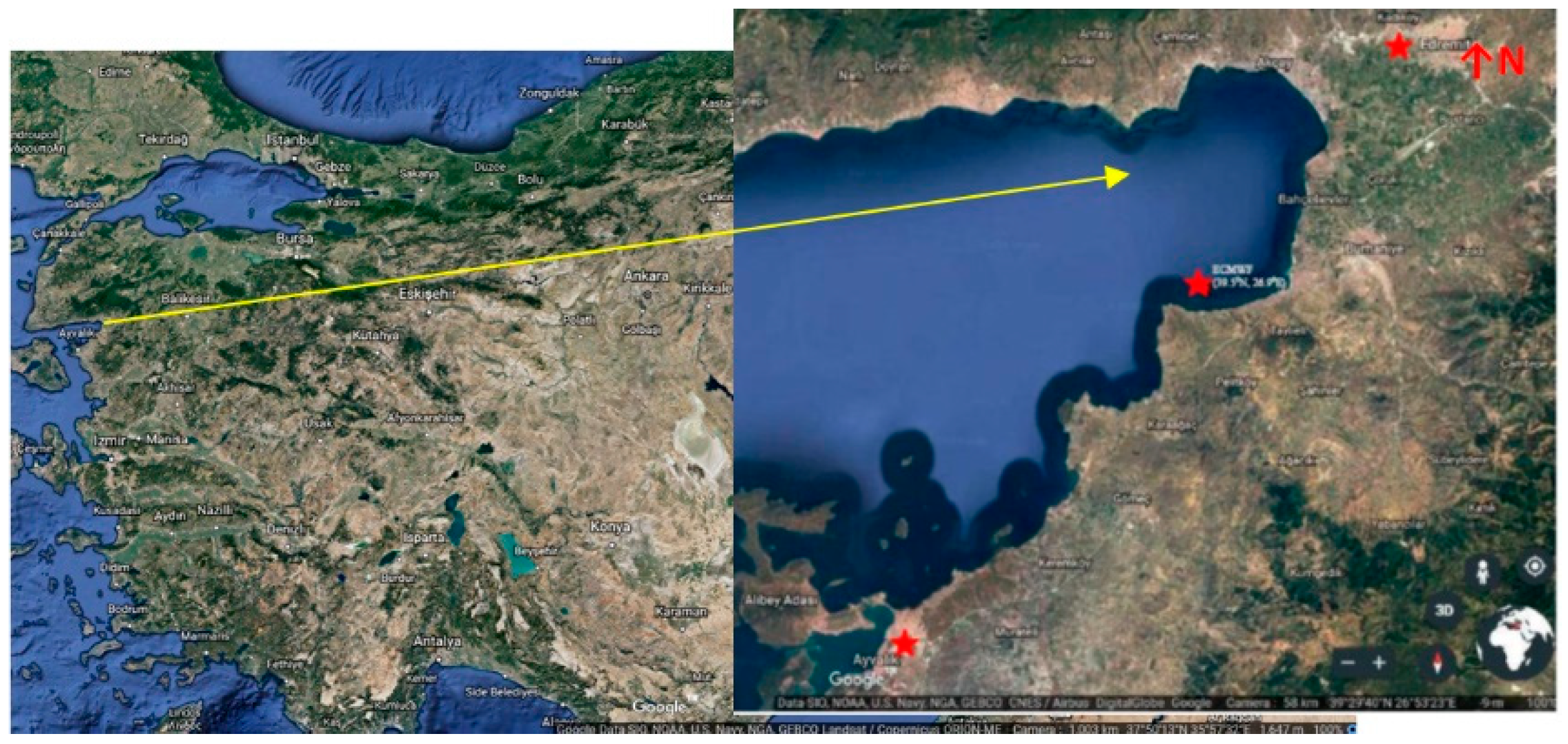
Edremit Bay is located in the Turkish northern Aegean Sea. It is the coastal water surrounded by the coastal plain between the Kaz Mountain and the Madra Mountain. Edremit Bay is gifted with gifted with the Kaz Mountain, which is called Ida in Greek mythology. The Kaz Mountain houses more than 800 species of plants. Furthermore, it is a unique home to 21 endemic species. This area was declared as a national park by the government in 1993 to provide official protection for the local flora and fauna. Edremit Bay has a fragile environment. The anthropogenic and natural coastal zone problems in Edremit Bay can be listed as follows: domestic wastewaters from hotels, secondary houses, holiday villages, wastewaters from olive oil production, conflicts between tourism and environmental conservation, urbanization, deterioration of seawater and freshwater quality, solid waste disposal, damage to coastal ecosystems, damage to river beds, the negative effects of basin erosion in the Kaz Mountain National Park, shoreline changes because of coastal erosion, negative effects of tourism facilities in the coastal zone, dense housing, loss of resources because of overutilization, and lack of infrastructure. The rapidly expanding coastal population in Edremit Bay in summer seasons threatens the sustainability of coastal resources as well as causing degradation of water quality in coastal areas [34,35]. The coastal zone of Edremit Bay is defined as a hot spot by the government [34]. The determination of long-term hydrodynamic and mixing processes in Edremit Bay is crucial for the National Coastal and Transitional Water Bodies Typology and Water Mass Studies in Turkey. The study area is located in the region of the sea outfall in the northwest of Edremit Bay (Figure 1).
4. Wind and Wave Climate
The wind roses provide the directional distribution of wind speeds. In this study, the wind roses were obtained from the measured wind data between the years 1970–2016 by the Ayvalık and Edremit State Meteorological Stations and from the predicted wind data of ECMWF (European Centre for Medium Range Weather Forecast) operational archive for coordinates of 39.50° N–26.90° E in Edremit Bay. Locations of Ayvalık and Edremit Meteorological Stations and the location of ECMWF operational archive for coordinates of 39.50° N–26.90° E are shown in Figure 1.
The wind roses from the Ayvalık and Edremit are given in Figure 2a,b, respectively. The wind characteristics are analyzed using the predicted wind data of ECMWF operational archive for coordinates of 39.50° N–26.90° E in Edremit Bay and the corresponding wind rose is shown in Figure 2c.
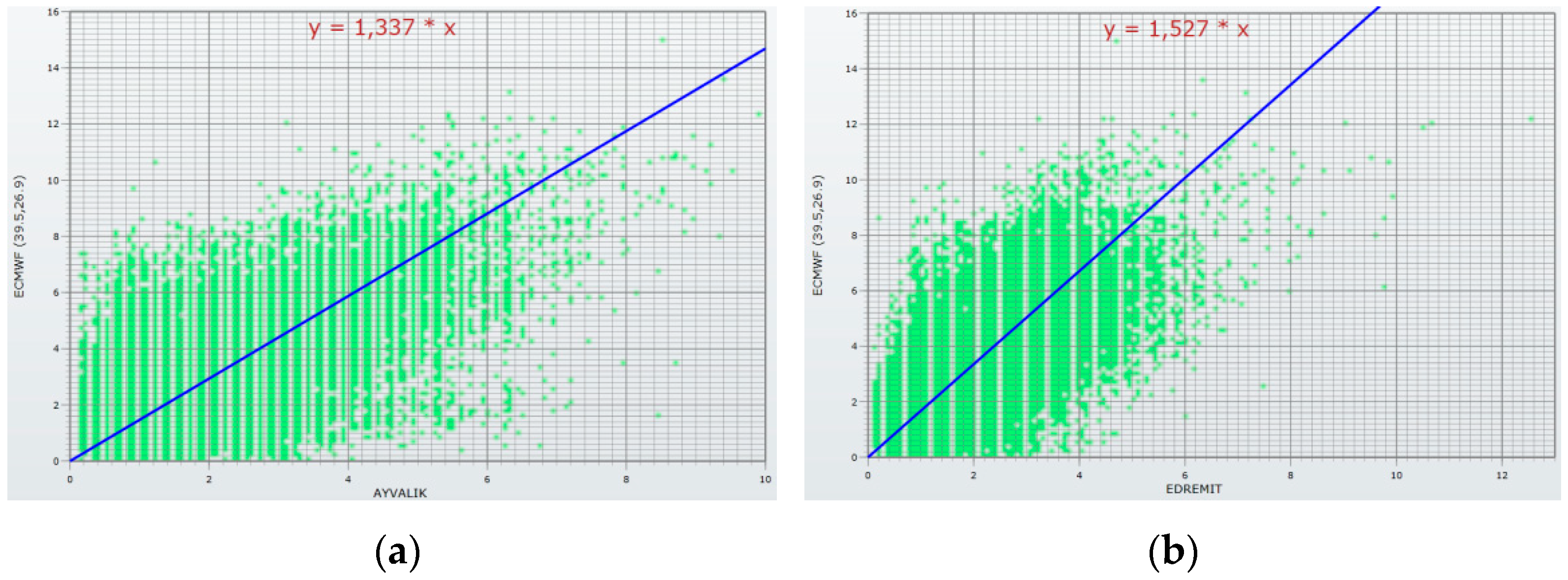
From wind measurements studies at the Ayvalık Meteorological Station, the interval of the dominant direction of the wind is determined as N–ENE. In these directions, results of long-term wind statistics indicate that the yearly average wind speed is 4 m/s, with a maximum of 13.9 m/s from a NE direction. The secondary wind direction interval is S–SE, with a yearly average for wind speed of 2.3 m/s, and a maximum of 10.6 m/s from a SSE direction. The interval of the tertiary wind direction is W–NNW, with a yearly average wind speed of 2.8 m/s, and a maximum of 12.7 m/s from a WNW direction. From wind measurements at the Edremit Meteorological Station, the interval of the dominant direction of the wind is determined as NNE–ESE. The yearly average wind speed is 2.8 m/s with a maximum of 9.5 m/s from an ENE direction based on the results of long term wind statistics. The interval of the secondary wind direction is WNW–SW, with a yearly average wind speed of 2.5 m/s and a maximum of 10.6 m/s from a WSW direction. From the wind data of ECMWF, the dominant wind direction was between NNE and ENE. In these directions, long-term wind statistics showed an average wind speed of 4.5 m/s, and with a maximum of 15.3 m/s from a NE direction. The secondary wind direction interval is S–SW, with a yearly average wind speed of 3.5 m/s and a maximum of 11.9 m/s from a SSW direction. The wind roses of the Ayvalık and Edremit Meteorological Stations, and ECMWF were in good agreement. The correlations of the wind velocities between land-based wind data and marine wind data are shown in Figure 3.
The ECMWF wind speed predictions were for 10 m above the sea surface. As expected, the values of the ECMWF wind speeds were greater than the land-based values. Therefore, it was decided that the wind data from the ECMWF operational archive were reliable and chosen to predict wave and current roses in this study.
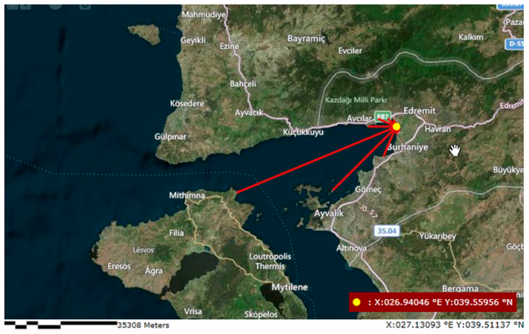
Fetch distances and directions, which were needed to study the long-term wave climate, are shown in Figure 4.
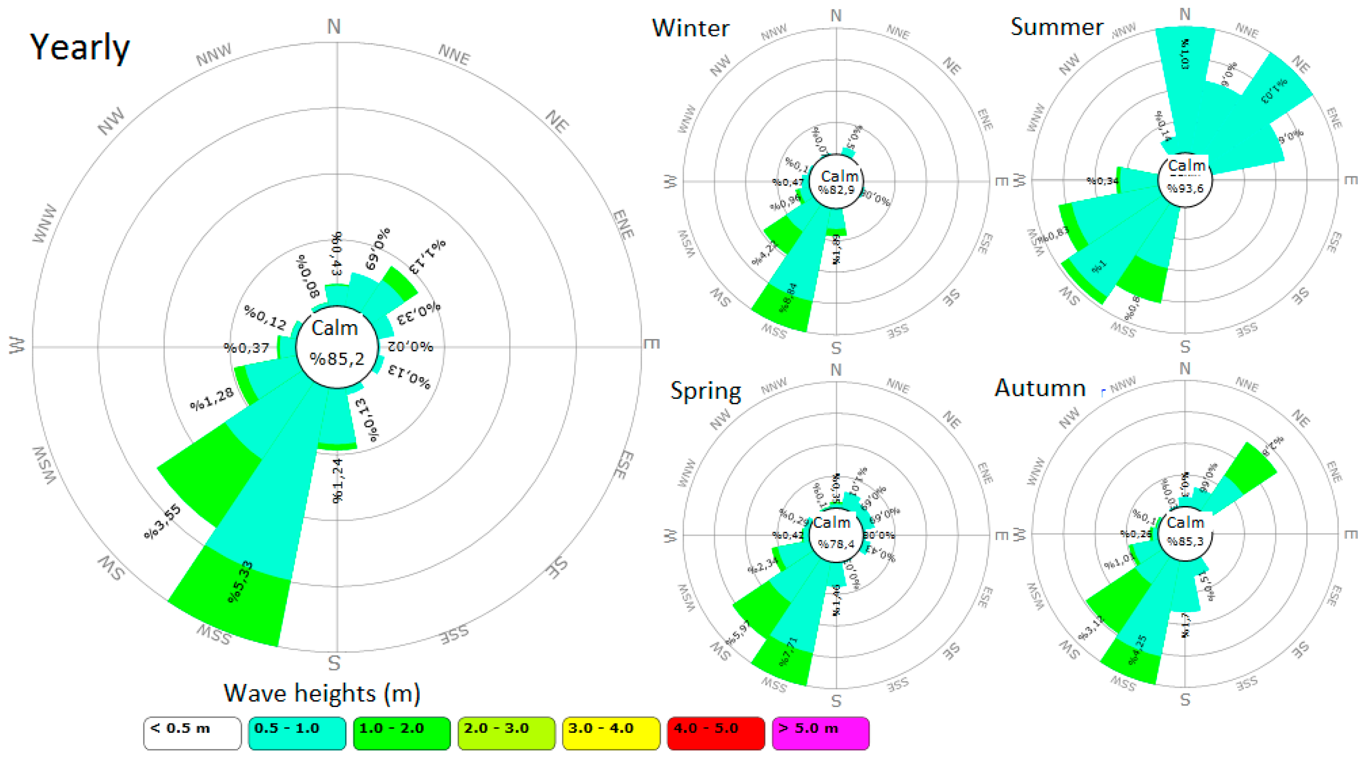
The CEM (Coastal Engineering Manual) method was utilized with the hourly averaged wind data to obtain the wave characteristics. The CEM method is a semi-empirical method based on dimensionless wave parameters [37]. Dimensionless wave height and period are defined using friction velocity and dimensionless time defined using wind speed [38,39]. As the location of the study area is an enclosed bay because of Mitilini Island, the CEM method was preferred. Moreover, it does not underestimate the wave heights. The cosine method was applied for the calculation of fetch distances. Because of the location of the study area, the directions for the longest fetch distances were between WNW–S as illustrated in Figure 4. Dominant wave directions are determined in the interval of WSW and S based on long-term wave statistics. The dominant wave direction is SSW. Predictions of the exceedance time and the probability distribution of the significant wave heights obtained from the data of ECMWF between the years 2000–2016 for the coordinate 39.50° N–26.90° E are given in Table 1.
Wave roses based on the results of long-term wave statistics from ECMWF data predictions are illustrated in Figure 5.
5. Current Pattern
In this study, currents because of winds, tides, breaking, and non-breaking waves were modeled using HYDROTAM-3D, which has hydrodynamic, transport, and turbulence model components. The model simulates transport processes because of tidal or nontidal forcing, that could be either barotropic or baroclinic. The hydrostatic pressure distribution and the Boussinesq approximation are used as simplifying approximations in the model. The Boussinesq approximation allows density variations to be entered into equations of motion and can be introduced by assuming that the basic state of the fluid is the state of no motion. The motion will increase only from density or pressure variations. The transport model component calculates the spatial and temporal distributions of water temperature and salinity. The variations in the water temperature and salinity affect the water density and, in turn, the velocity field [14,17]. The water depth, water salinity, water temperature, and discharge are taken automatically from the database and transferred as input to HYDROTAM-3D. The simulations begin with the assumption of still water level without currents at the initial time. In HYDROTAM-3D, the M2 tide, which is found along the Turkish coasts, is defined. The wave height and the period of the tide were taken as 50 cm and 12.42 h, respectively. The convection, the velocity of the tide, and the change of the water level were calculated with the radiation type of boundary condition at the offshore boundary [29,32].
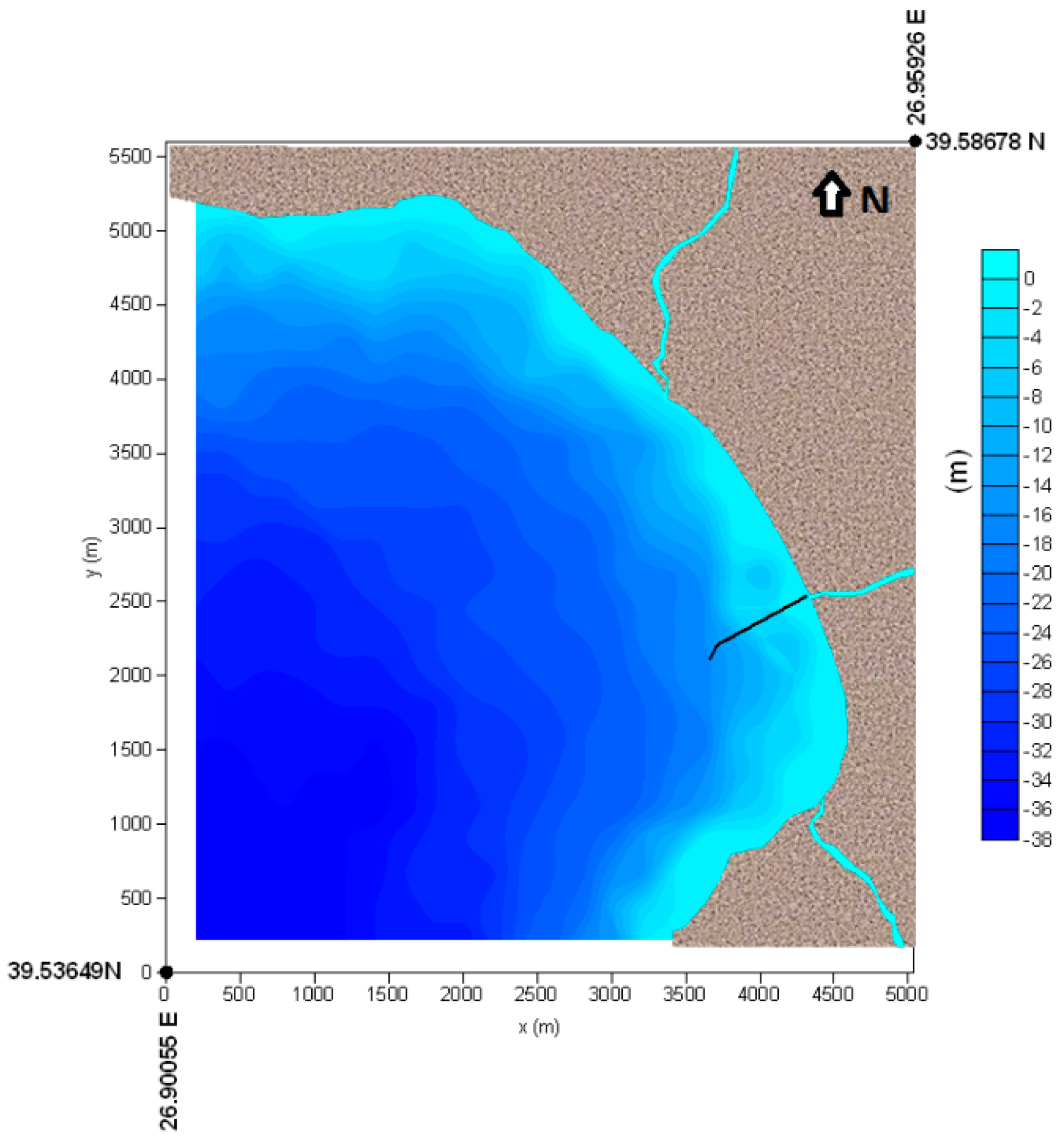
Water depths and the location of the outfall pipe are shown in Figure 6. Circulation in coastal regions is typically irregular and turbulent. In the model, the connection between average motion and turbulent motion was merged with mass transport because of vertical and horizontal eddy viscosities and vertical and horizontal eddy diffusion. Vertical and horizontal turbulence differ where the surface area of a coastal region, like Edremit Bay, is significantly great relative to the water depth. This difference results in an anisotropic condition, therefore, different horizontal and vertical eddy viscosities come into prominence for the simulations. An isotropic k-ε model was used for calculation of vertical eddy viscosities and the Smagorinsky turbulence model was used for horizontal eddy viscosities to compensate the difference.
Current roses of the study area, presented in Figure 7, are based on the six hourly wind data of ECMWF for the coordinates of 39.50° N–26.90° E in Edremit Bay between 2012–2016. The server used in the simulations was HP DL70 8 Cores Xeon CPU, 32 GB Memory, 4 TB Disk. The simulation of the current pattern for each year took nearly 2–2.5 h using this server. After the outputs of the currents for each year were combined, and the current rose was obtained. At the sea surface, the interval of the dominant direction of the current was determined as WNW–WSW and the secondary current direction was NE, as seen in Figure 7a.
The seasonal occurrence frequencies of the winds from different directions are listed in Table 2. In the hydrodynamic model, it was observed that wind velocities that were equal or greater than 10 m/s induced currents with a velocity of 25 cm/s or greater at the surface, and if wind velocity was 2 m/s or less, then currents occurred with a velocity 5 cm/s or less. In the coastal area of Edremit Zeytinli Sea Outfall, current velocities that were less than 5 cm/s were expected 98% of the time.
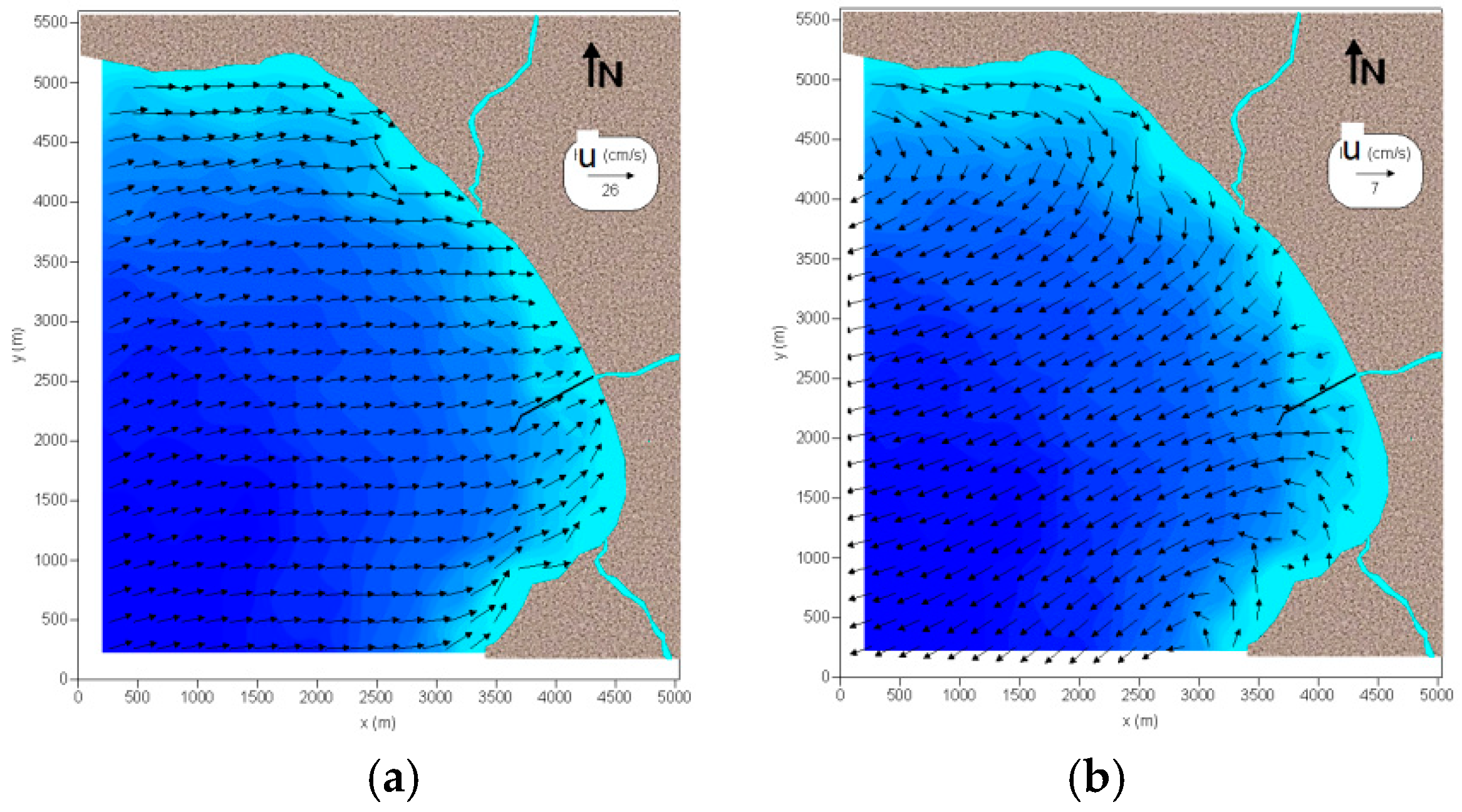
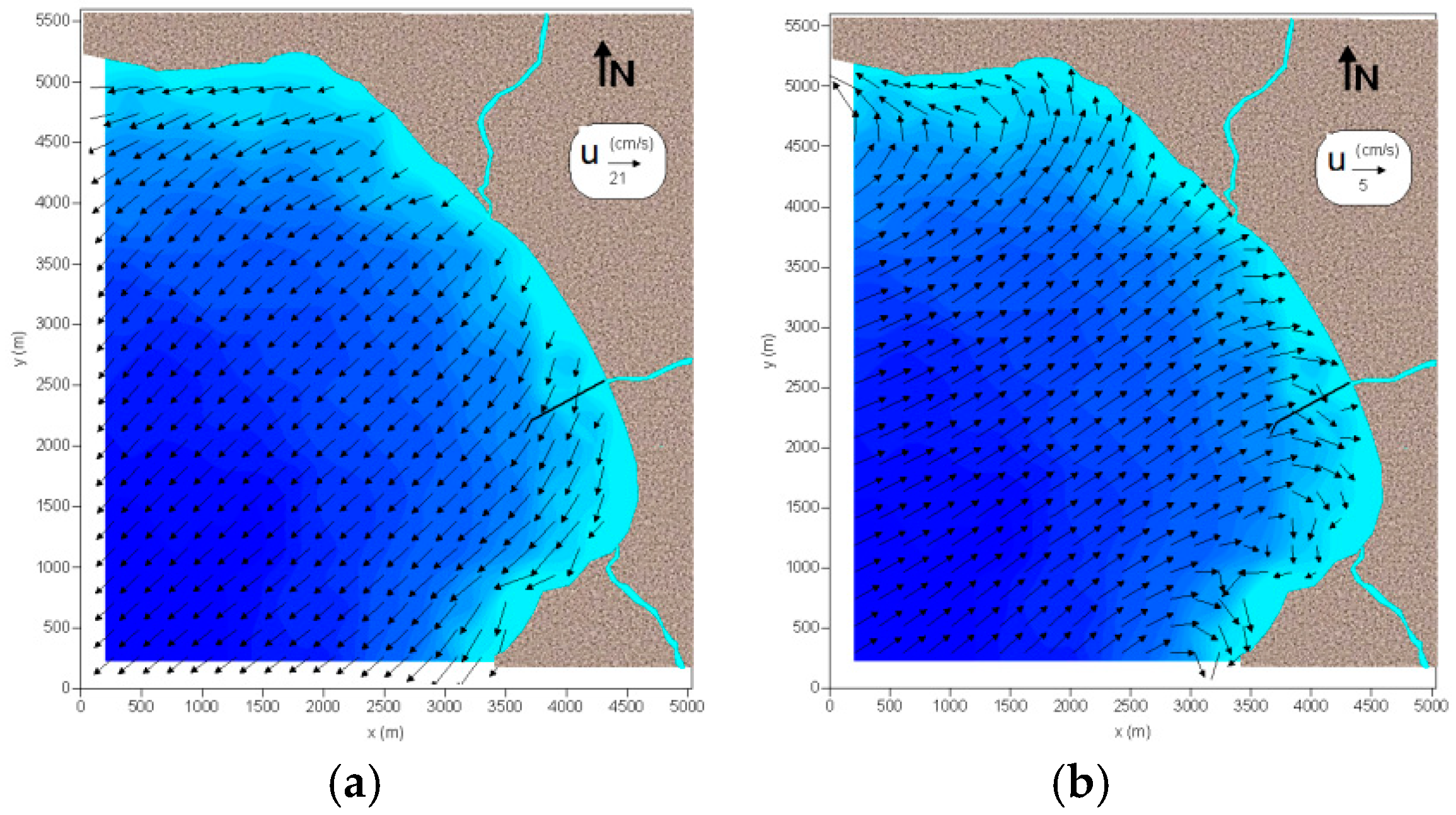
The average salinity is 38.11 ppt and the average temperature of the sea water is 18.47 °C based on the measurements [40]. These values are considered in the calculations of density of the ambient sea water. Sea water density is assumed constant along water column and calculated as ρa = 1028 kg/m3. The temperature of sea water, salinity, and density were taken as constant in the numerical model. The steady state circulation patterns at the surface and bottom layers under the shear forcing of wind blowing from WSW, WNW, and NE at 10 m/s are shown in Figure 8, Figure 9 and Figure 10.
It was observed that under the effect of westerly winds, there occurred surface currents from the west to east direction in the study field, whereas under the effect of northerly winds, surface currents were from the north to south direction. Under the effect of the barotropic pressure gradient, current directions turned to the opposite of the surface currents towards the sea bottom. Surface current speeds were about 20–30 cm/s and decreased almost four times in the bottom layer.
6. Modeling of Pollutant Transport
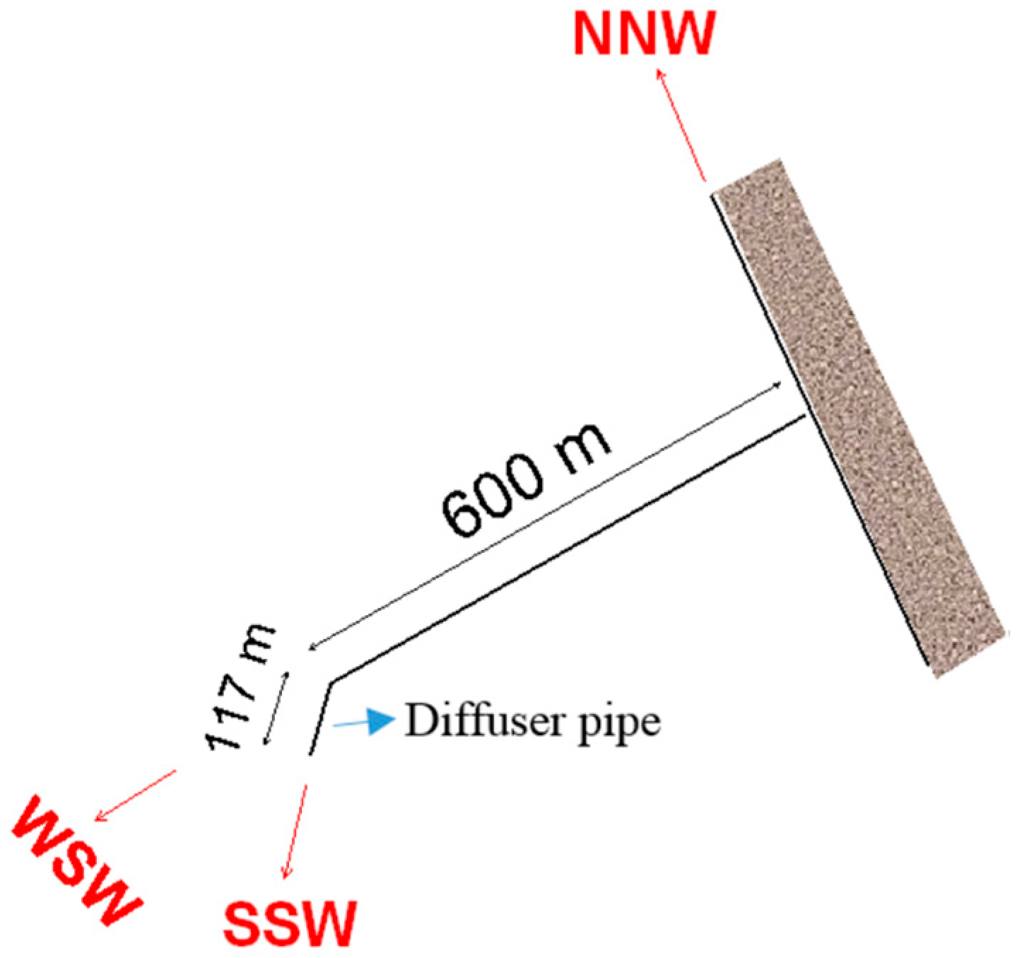
The physical properties of the sea outfall of Edremit that were used as data for near-field and far-field dilutions modeling of the pollutant are presented in Table 3. The length of the feeder pipe was 600 m. The sea outfall system is illustrated schematically in Figure 11 showing the alignments of the feeder pipe and the diffuser.
7. Results and Discussion
Near-field dilution modeling is affected by wastewater discharge, changes in density, current velocity, angle between current directions, and diffuser pipes. CORMIX2 was used for the near-field calculations. CORMIX2 is the submodule of CORMIX for multiport diffusers [19]. Water depths were shallower than 20 m in the study area. Density changes in water column are neglected in hydrodynamic studies as the greatest change in density occurs in the summer season, and it is understood that is < 0.02. The small density difference at the discharge level does not cause trapping of the pollutant cloud. In each season, pollutant cloud reaches the water surface, therefore, near-field mixing process ends at the water surface. The design parameters used in near-field dilution modeling are presented in Table 3. The simulation of the near-field dilution by CORMIX2 takes a couple of seconds.
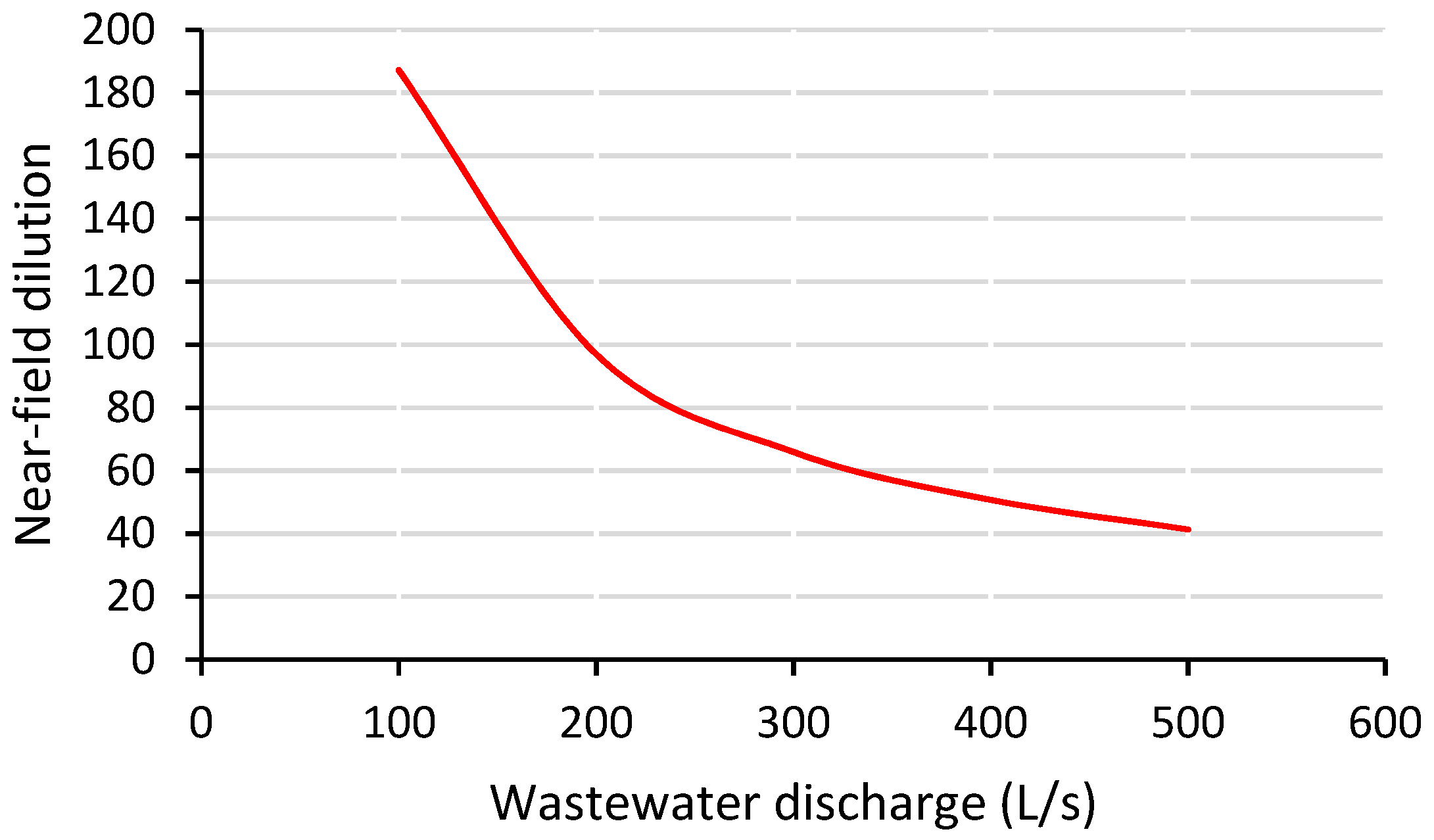
The effect of wastewater discharge on the near-field dilution is shown in Figure 12. When the current velocity is 5 cm/s, it indicates still water. The current velocity was taken as u = 10 cm/s so that the current effect can be considered although it had a low value. The near-field dilution was modeled for γ = 90° (angle between current direction and diffuser pipe). As the wastewater discharge increased, the near-field dilution decreased. Near-field dilution was 41.5 when the discharge was 500 L/s. This discharge was twice as much as the actual wastewater discharge of the sea outfall. As the discharge increased, the asymptotic behavior of the curve began. The near-field dilution should be greater than 40 to satisfy Turkish near-field dilution requirements [41]. The results, which are shown in Figure 12, fulfill this condition.
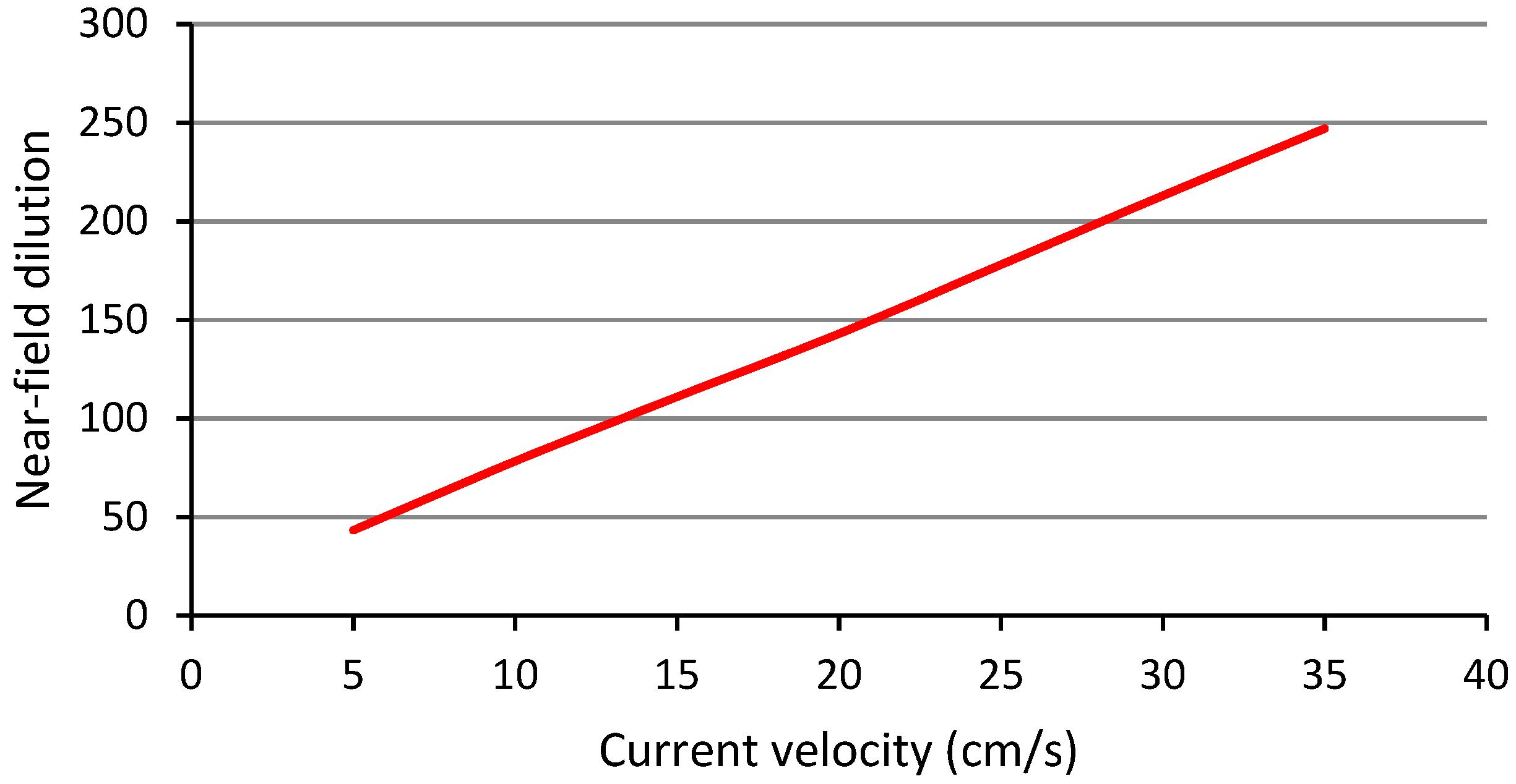
The relationship between current velocity and near-field dilution is studied and shown in Figure 13. Wastewater discharge (Q) and the angle between current direction and diffuser pipe (γ) are taken as 250 L/s and γ = 90°, respectively. If the current velocity is 5 cm/s or less, it is assumed that ambient water is still. It is the worst condition for dilution. In this study, when the current velocity was 5 cm/s, the near-field dilution was 43.3 and it satisfied Turkish near-field dilution requirements. Near-field dilution increased with increasing current velocity and near-field dilution was greater than 40 as shown in Figure 13.
After the pollutant cloud reaches the water surface because of near-field dilution, far-field dilution began under the effect of currents. Far-field dilution was simulated by HYDROTAM-3D. The pollutant cloud spread through advection, turbulent diffusion, and dispersion, and bacteria disappeared because they died. T90 was taken as 1.5 h in summer and 2.5 h in winter in numerical modeling.
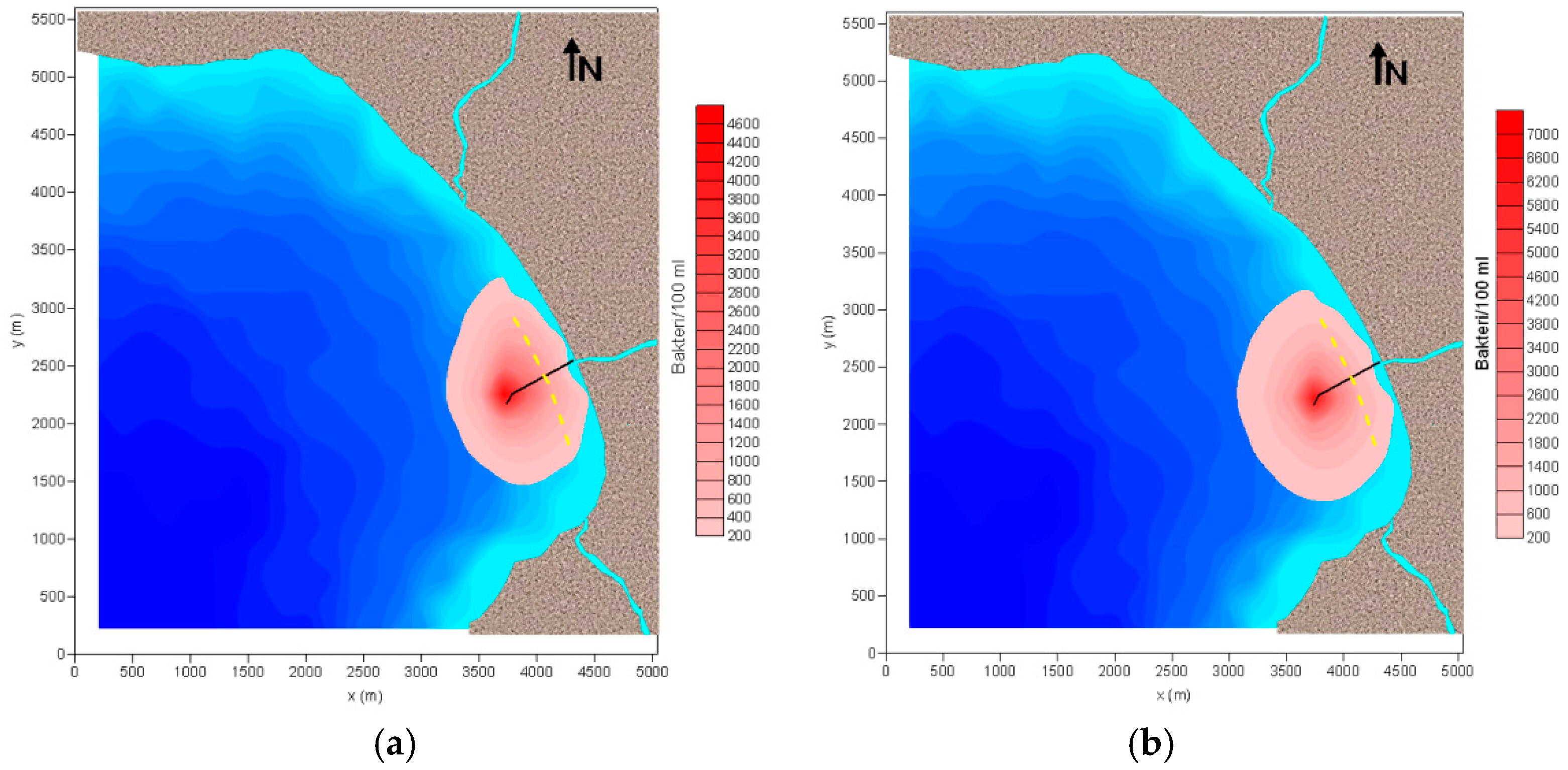
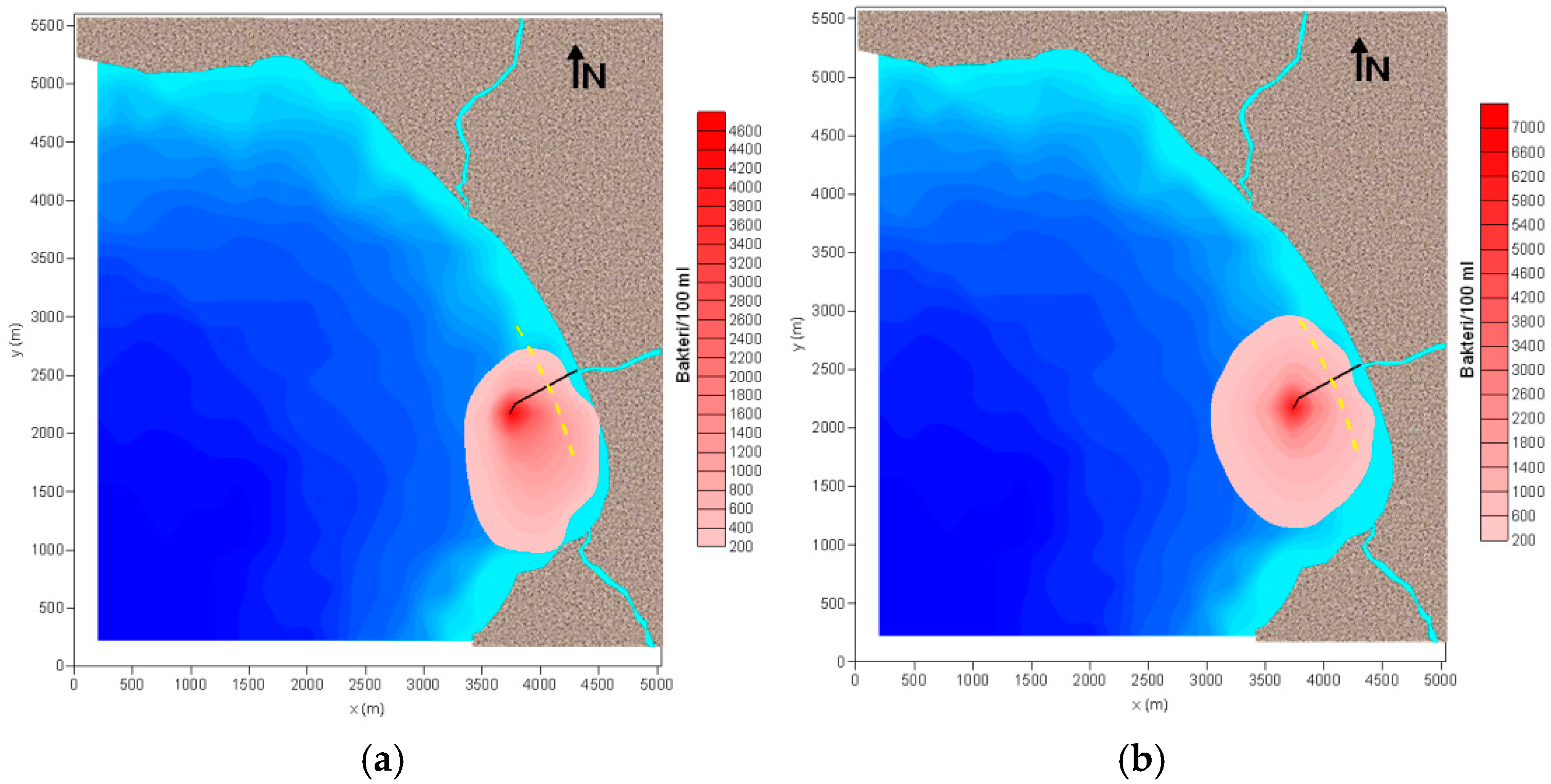
As seen from the long-term current roses in Figure 7, the interval of the dominant direction of the current was determined as WNW–WSW and the secondary current direction was NE at the sea surface. Therefore, the steady state spreading of the pollutant cloud because of far-field dilution under the influence of hydrodynamics corresponding to the wind blowing from WSW, WNW, and NE at 10 m/s and 2 m/s, selected from the time series analysis are given in Figure 14, Figure 15 and Figure 16, respectively. The solid black line is the diffuser pipe line and the dotted yellow line is the boundary of shore protection zone in these figures. The shore protection zone is the preserved area of human contact. The total dilution should be sufficient to yield less than 1000 total coliform per 100 mL for 90% of the time when sampled in the shore protection zone based on the Turkish Water Pollution Control Regulations [41]. The scenarios were prepared depending on the occurrence frequencies of currents caused by blowing wind from different directions presented in Table 2. The maximum number of total bacteria was about 4500–5000 bac /100 mL under the effect of winds with a speed of 10 m/s, whereas the maximum number of total bacteria was about 6000–7000 bac /100 mL under the effect of winds with a speed 2 m/s, as seen in Figure 14, Figure 15 and Figure 16. As the wind speed increased, the current speed increased and it brought a dramatic rise of near- and far-field dilutions. The pollutant distribution under the effect of the wind blowing from WNW is highly risky depending on the coastal alignment. It transports the pollutants from the wastewater to the shallow zone. The wind blowing from the NE causes the pollutants to disperse offshore.
8. Conclusions
In this study, the wind and wave climates, the long-term wave statistic, the wind-tide-wave-wave breaking induced currents, and the far-field dilution of the pollutant cloud for the coastal area of Edremit Bay were modeled numerically with the 3D hydrodynamic transport model HYDROTAM-3D. Near-field dilution of the pollutants were modeled with the CORMIX. The wind rose providing the directional distribution of the wind speeds was obtained from the measured wind data between the years 1970–2016 of the Edremit and Ayvalık State Meteorological Stations. From wind measurements of the Edremit Meteorological Station, the interval of the dominant wind direction was determined as NNE–ESE. The yearly average wind speed was 2.8 m/s, with a maximum of 9.5 m/s from an ENE direction, based on the results of long-term wind statistics. From the wind measurements of the Ayvalık Meteorological Station, the interval of dominant direction of the wind is N and ENE. In these directions, results of long-term wind statistics show that the yearly average wind speed is 4m/s with a maximum of 13.9 m/s from a NE direction. Wind characteristics were analyzed using the observed wind data of ECMWF (European Centre for Medium Range Weather Forecast) for the coordinates 39.50° N–26.90° E in Edremit Bay between 2000 and 2016 to obtain wave predictions. From the ECMWF wind data, the dominant wind direction are NNE and ENE. In these directions, the results of long-term wind statistics showed the yearly average value of wind speed to be 4.5 m/s with a maximum of 15.3 m/s from a NE direction. The wind roses of the Ayvalık and Edremit Meteorological Stations and ECMWF were in good agreement. Predictions of wave and current roses were based on the wind data of ECMWF. Wave roses show that the dominant wave propagation direction was between WSW–S. The interval of the dominant direction of the current at the sea surface was obtained as WNW–WSW, and the secondary current direction was NE. The coastal alignment was along NNW–SSE. The winds blowing from WSW to ENE, and the winds from the NE caused drift from NE to SW. The current velocities were predicted to be 25 cm/s at the water surface and 5 cm/s at the bottom, based on current measurements. Ninety-eight percent of the time, current velocity was smaller than 5 cm/s in the coastal area of the sea outfall. Water depths were less than 20 m in the study area. The density difference along the water column was neglected. The low density difference at the discharge depth did not influence trapping of the pollutant cloud. In all seasons, the pollutant cloud reached the surface, where near-field dilution ended.
The effects of the wastewater discharge and current velocity on the near-field dilution were studied. It was confirmed, for the conditions used in this study, that near-field dilution was greater than 40. As current speed increased or wastewater discharge decreased, near-field dilution increased. Far-field dilution began at the water surface. The width of the shore protection zone was taken as 300 m. The model results show that total bacteria were less than 1000 bac/100mL 98% of the time in the shore protection zone. With respect to the results of the near-field and far-field dilution modeling, it can be stated that the sea outfall of the Edremit–Zeytinli meets the legal regulations [41].
Under the effects of winds with a speed 10 m/s, the travel times of the pollutant for the near-field and far-field dilution were approximately 10 min and 1 h, respectively. When the speed of the winds decreased and also the current velocity decreased, the travel times of the pollutant for the near-field and far-field dilution increased. Under the effects of winds with a speed 2 m/s, the travel times of the pollutant for the near-field and far-field dilution increased approximately to 25 min and 4 h, respectively.
The numerical models become more important especially in the lack of the field measurements in the environmental studies. They can serve as a powerful design tool and can be achieved in a decision support system.
The applications of two different previously calibrated complex numerical models with several experimental and field studies as referenced in the field of coastal engineering have been presented. The understanding of long-term hydrodynamic and mixing behaviors by such modelling studies in coastal waters are quite important in the typology and water mass classification studies, since in most of the cases the long-term measurements covering such large extended bodies do not yet exist. Therefore, numerical models and their large extent applications as presented are important tools in the coastal water management studies. Numerical model applications for the enclosed coastal waters of Edremit Bay are also quite important in National Coastal and Transitional Water Bodies Typology and Water Mass Studies in Turkey that are still in progress.
Funding
CORMIX is funded by the project entitled “Modeling of Near Field Dilution for Saline and/or Heated Discharges” (Report No: 114Y806) of TÜBİTAK 1002 Programme (The Scientific and Technological Research Council for Turkey).
Acknowledgments
This study was supported by DLTM Environmental Software Technologies Limited. Special thanks are extended to Lale Balas who supported the modelling studies of HYDROTAM-3D as a part of National Coastal Water Bodies Typology and Water Mass Studies in Turkey.
Conflicts of Interest
The author declares no conflict of interest.
Nomenclature
| Buoyant gravitational acceleration | |
| Effluent density | |
| Vertical ambient distribution | |
| Reference density | |
| C | Pollutant concentration |
| Dx | Turbulent diffusion coefficients in x-direction |
| Dy | Turbulent diffusion coefficients in y-direction |
| Dz | Turbulent diffusion coefficients in z-direction |
| kp | Decay rate of pollutant |
| Ss | Concentration at the farthest point of near-field region (pollutant source) |
| u | Velocities in s (axial) direction of the buoyant jet |
| v | Velocity in r (transverse) direction of the buoyant jet |
| bac | Bacteria |
References
- Malcangio, D.; Ben Meftah, M.; Mossa, M. Physical Modelling of Buoyant Effluents Discharged into a Cross Flow. In Proceedings of the 2016 IEEE Workshop on Environmental, Energy and Structural Monitoring Systems, Bari, Italy, 13–14 June 2016. [Google Scholar]
- Malcangio, D.; Petrillo, A.F. Modeling of Brine Outfall at the Planning Stage of Desalination Plants. Desalination 2010, 254, 114–125. [Google Scholar] [CrossRef]
- Ben Meftah, M.; Malcangio, D.; De Serio, F. Vertical Dense Jet in Flowing Current. Environ. Fluid Mech. 2018, 18, 75–96. [Google Scholar] [CrossRef]
- Tian, X.; Roberts, P.J.W.; Daviero, G.J. Marine wastewater discharges from multiport diffusers I: Unstratified stationary water. J. Hydraul. Eng. 2004, 130, 1137–1146. [Google Scholar] [CrossRef]
- Roberts, P.J.W.; Salas, H.J.; Reiff, F.M.; Libhaber, M.; Labbe, A.; Thomson, J.C. Marine Wastewater Outfalls and Treatment Systems, 2nd ed.; IWA Publishing: London, UK, 2011; pp. 51–134. ISBN 9781843391890. [Google Scholar]
- Wood, I.R.; Bell, R.G.; Wilkinson, D.L. Ocean Disposal of Wastewater, Advanced Series on Ocean Engineering; World Scientific Publishing Co. Pte. Ltd.: Singapore, 1993; Volume 8, pp. 178–214. ISBN 978-981-02-0956-8. [Google Scholar]
- Malcangio, D.; Mossa, M. A Laboratory Investigation into the Influence of a Rigid Vegetation on the Evolution of a Round Turbulent Jet Discharged within a Cross Flow. J. Environ. Manag. 2016, 173, 105–120. [Google Scholar] [CrossRef]
- Malcangio, D.; Melena, A.; Damiani, L.; Mali, M.; Saponieri, A. Numerical Study of Water Quality Improvement in a Port through a Forced Mixing System. WIT Trans. Ecol. Environ. 2017, 220, 69–80. [Google Scholar]
- Mali, M.; Malcangio, D.; Dell’Anna, M.M.; Damiani, L.; Mastrorilli, P. Influence of Hydrodynamic Features in the Transport and Fate of Hazard Contaminants within Touristic Ports. Case study: Torre a Mare (Italy). Heliyon 2018, 4, e00494. [Google Scholar] [CrossRef] [PubMed]
- Montessori, A.; Prestininzi, P.; La Rocca, M.; Malcangio, D.; Mossa, M. Two Dimensional Lattice Boltzman Numerical Simulation of a Buoyant Jet. In Proceedings of the 4th IAHR Europe Congress, Liege, Belgium, 27–29 July 2016. [Google Scholar]
- Bleninger, T. Coupled 3D Hydrodynamic Models for Submarine Outfalls: Environmental Hydraulic Design and Control of Multiport Diffusers. Ph.D. Thesis, Hydromechanic Institute, Karlsruhe University, Karlsruhe, Germany, 2006. [Google Scholar]
- Daviero, G.J.; Roberts, P.W.J. Marine wastewater discharges from multiport diffusers III: Stratified stationary water. J. Hydraul. Eng. 2006, 132, 404–410. [Google Scholar] [CrossRef]
- Doneker, R.L.; Jirka, G.H. CORMIX User Manual: A Hydrodynamic Mixing Zone Model and Decision Support System for Pollutant Discharges into Surface Waters; U.S. Environmental Protection Agency: Washington, DC, USA, 2007; pp. 7–110.
- Frick, W.E. Visual plumes mixing zone modelling software. Environ. Model. Softw. 2004, 19, 645–654. [Google Scholar] [CrossRef]
- Bombardelli, F.A.; Cantero, M.I.; Buscaglia, G.C.; García, M.H. Comparative study of convergence of CFD commercial codes when simulating dense underflows. Mecánica Comput. 2004, 23, 1187–1199. [Google Scholar]
- Kaminski, E.; Tait, S.; Carzzo, G. Turbulent entrainment in jets with arbitrary buoyancy. J. Fluid Mech. 2005, 526, 361–376. [Google Scholar] [CrossRef]
- Choi, K.W.; Lee, J.H.W. Distributed entrainment sink approach for modeling mixing and transport in the intermediate field. J. Hydraul. Eng. 2007, 133, 804–815. [Google Scholar] [CrossRef]
- Morelissen, R.I.; van der Kaaij, T.; Bleninger, T. Dynamic coupling of near-field and far-field models for simulating effluent discharges. Water Sci. Technol. 2013, 67, 2210–2220. [Google Scholar] [CrossRef]
- Naidu, V.S. Estimation of near-field and far-field dilutions for site selection of effluent outfall in a coastal region-a case study. J. Coast. Res. 2013, 29, 1326–1340. [Google Scholar] [CrossRef]
- Mixing Zone Model (CORMIX). Available online: www.mixzon.com (accessed on 15 September 2018).
- Bleninger, T.; Jirka, G.H. Modelling and Environmental Sound Management of Brine Discharges from Desalination Plant. Desalination 2008, 221, 585–597. [Google Scholar] [CrossRef]
- Jirka, G.H. Integral Model for Turbulent Buoyant Jets in Unbounded Stratified Flows Part 2: Plane Jet Dynamics Resulting from Multiport Diffuser Jets. Environ. Fluid Mech. 2006, 6, 43–100. [Google Scholar] [CrossRef]
- Maia, L.P.; Bezerra, M.O.; Pinheiro, L.; Redondo, J.M. Application of the Cormix model to assess environmental impact in the coastal area: An example of the ocean disposal system for sanitary sewers in the city of Fortaleza (Ceará, Brazil). J. Coast. Res. 2011, 64, 922–926. [Google Scholar]
- Schreiner, S.; Krebs, T.A.; Strebel, D.E.; Brindley, A. Testing the CORMIX Model Using the Thermal Plume Data from Four Maryland Power Plants. Environ. Modell. Softw. 2002, 17, 321–331. [Google Scholar] [CrossRef]
- Yılmaz, N.; Inan, A. Modeling of near field dilution of heated discharges of sea outfalls. J. Fac. Eng. Archit. Gazi Univ. 2018, 33, 875–886. [Google Scholar]
- Balas, L. Simulation of pollutant transport in Marmaris Bay. In China Ocean Engineering; Nanjing Hydraulics Research Institute (NHRI): Nanjing, China, 2002; Volume 15, pp. 565–578. [Google Scholar]
- Yılmaz, N.; Cebe, K.; Yıldırım, P.; İnan, A.; Balas, L. The need for the integration of land use planning and water quality modeling in the case of Fethiye Bay. J. Polytech. 2017, 2, 427–435. [Google Scholar]
- Cebe, K.; Balas, L. Monitoring and modeling land-based marine pollution. Reg. Stud. Mar. Sci. 2018, 24, 23–39. [Google Scholar] [CrossRef]
- Balas, L.; Ozhan, E. Three dimensional modelling of stratified coastal waters. J. Estuar. Coast. Shelf Sci. 2001, 54, 75–87. [Google Scholar] [CrossRef]
- Balas, L.; Inan, A.; Numanoğlu Genç, A. Modelling of dilution of thermal discharges in enclosed coastal waters. Res. J. Chem. Environ. 2013, 17, 82–89. [Google Scholar]
- Cebe, K.; Balas, L. Water quality modelling in Kaş Bay. Appl. Math. Model. 2016, 40, 1887–1913. [Google Scholar] [CrossRef]
- Yılmaz, N. Modeling of wind climate, wave climate and current pattern in Samsun Bay coastal waters. J. Fac. Eng. Archit. Gazi Univ. 2018, 33, 279–297. [Google Scholar]
- Three Dimensional Hydrodynamic Transport Model (HYDROTAM-3D). Available online: http://www.hydrotam3d.com (accessed on 1 September 2018).
- General Directorate of Water Management Staff, Action Plan of North Aegean Basin; Ministry of Forestry and Water Affairs: Ankara, Republic of Turkey, 2014; pp. 80–124.
- Irtem, E.; Kabdaşlı, S.; Azbar, N. Coastal zone problems and environmental strategies to be implemented at Edremit Bay, Turkey. Environ. Manag. 2005, 36, 37–47. [Google Scholar] [CrossRef] [PubMed]
- Google Earth. 2018. Available online: https://www.google.com/earth/ (accessed on 1 July 2018).
- Coastal Engineering Research Center Staff. Coastal Engineering Manual (CEM) Part II; Coastal Engineering Research Center, Department of the Army, US Army Corps of Engineers: Washington, DC, USA, 2006; ISBN 9781782661900. [Google Scholar]
- Etemad-Shadidi, A.; Kazeminezhad, M.H.; Mousavi, S.J. On the wave predictions of wave parameters using simplified methods. J. Coast. Res. 2009, SI56, 505–509. [Google Scholar]
- Kazeminezhad, M.H.; Etemad-Shadidi, A.; Mousavi, S.J. Testing of CEM wave prediction model for Lake Ontario. In Proceedings of the 6th International Conference on Hydrodynamics, Perth, Western Australia, 24–26 November 2004; Cheng, L., Yeow, K., Eds.; Taylor & Francis Group: Boca Raton, FL, USA, 2004. [Google Scholar]
- Ozturk, I.; Eroglu, V.; Altay, A.; Bayhan, H. Oceanographic Research Report for Edremit- Zeytinli Sea Outfall and Refinement Unit; Turkey’s Bank of Provinces: Turkey, 1992; pp. 32–55. (In Turkish) [Google Scholar]
- Regulation of Water Pollution Control, (RWPC); No. 25687, Clause 35; Official Gazette: Ankara, Turkey, 2004. (In Turkish)
Figure 1.
Geographical location of the study area in Edremit Bay [36].
Figure 1.
Geographical location of the study area in Edremit Bay [36].

Figure 2.
Wind rose based on hourly wind measurements for 1970–2016: (a) Ayvalık Meteorological Station; (b) Edremit Meteorological Station; and (c) wind rose based on wind predictions with 6 h intervals for 2000–2016 from European Centre for Medium Range Weather Forecast (ECMWF) operational archive for coordinates of 39.50 °N–26.90 °E [33].

Figure 3.
Correlations of wind velocities (m/s) between: (a) Ayvalık Meteorological Station and ECMWF operational archive for coordinates of 39.50° N–26.90° E; (b) Edremit Meteorological Station and ECMWF operational archive for coordinates of 39.50° N–26.90° E [33].
Figure 3.
Correlations of wind velocities (m/s) between: (a) Ayvalık Meteorological Station and ECMWF operational archive for coordinates of 39.50° N–26.90° E; (b) Edremit Meteorological Station and ECMWF operational archive for coordinates of 39.50° N–26.90° E [33].

Figure 4.
Fetch distances according to directions [33].
Figure 4.
Fetch distances according to directions [33].

Figure 5.
Wave roses [33].
Figure 5.
Wave roses [33].

Figure 6.
Water depth (m) and the location of outfall pipe.

Figure 7.
Current roses: (a) sea surface layer and (b) bottom layer from ECMWF for 2012–2016 for coordinates 39.50° N–26.90° E [33].
Figure 7.
Current roses: (a) sea surface layer and (b) bottom layer from ECMWF for 2012–2016 for coordinates 39.50° N–26.90° E [33].

Figure 8.
Current pattern: (a) sea surface layer and (b) bottom layer, for wind blowing from WSW with speed 10 m/s at the steady state [33].
Figure 8.
Current pattern: (a) sea surface layer and (b) bottom layer, for wind blowing from WSW with speed 10 m/s at the steady state [33].

Figure 9.
Current pattern: (a) sea surface layer and (b) bottom layer, for wind blowing from WNW with speed 10 m/s at the steady state [33].
Figure 9.
Current pattern: (a) sea surface layer and (b) bottom layer, for wind blowing from WNW with speed 10 m/s at the steady state [33].

Figure 10.
Current pattern: (a) sea surface layer and (b) bottom layer, for wind blowing from NE with speed 10 m/s at the steady state [33].
Figure 10.
Current pattern: (a) sea surface layer and (b) bottom layer, for wind blowing from NE with speed 10 m/s at the steady state [33].

Figure 11.
Sea outfall system.

Figure 12.
The effect of wastewater discharge on near-field dilution [20].
Figure 12.
The effect of wastewater discharge on near-field dilution [20].

Figure 13.
Effect of current velocity on near-field dilution [20].
Figure 13.
Effect of current velocity on near-field dilution [20].

Figure 14.
Distribution of the pollutant cloud caused by the wind blowing from WSW at: (a) 10 m/s and (b) 2 m/s [33].
Figure 14.
Distribution of the pollutant cloud caused by the wind blowing from WSW at: (a) 10 m/s and (b) 2 m/s [33].

Figure 15.
Distribution of the pollutant cloud caused by the wind blowing from WNW at: (a) 10 m/s and (b) 2 m/s [33].
Figure 15.
Distribution of the pollutant cloud caused by the wind blowing from WNW at: (a) 10 m/s and (b) 2 m/s [33].

Figure 16.
Distribution of the pollutant cloud caused by the wind blowing from NE at: (a) 10 m/s and (b) 2 m/s [33].
Figure 16.
Distribution of the pollutant cloud caused by the wind blowing from NE at: (a) 10 m/s and (b) 2 m/s [33].


Table 1.
Exceedance time interval and the probability distribution of significant wave heights (Hs) of ECMWF data for 2000–2016 [33].
Table 1.
Exceedance time interval and the probability distribution of significant wave heights (Hs) of ECMWF data for 2000–2016 [33].
| Direction | Distribution Equation | 1 h/year | 5 h/year | 10 h/year |
|---|---|---|---|---|
| Hs (m) | Hs (m) | Hs (m) | ||
| WNW | Hs = −1.11 − 0.268ln(p(H)) | 1.3 | 0.9 | 0.7 |
| W | Hs = −0.714 − 0.225ln(p(H)) | 1.3 | 1.0 | 0.8 |
| WSW | Hs = −0.708 − 0.283ln(p(H)) | 1.9 | 1.4 | 1.2 |
| SW | Hs = −0.781 − 0.424ln(p(H)) | 3.0 | 2.4 | 2.1 |
| SSW | Hs = −0.404 − 0.323ln(p(H)) | 2.5 | 2.0 | 1.8 |
| S | Hs = −0.479 − 0.233ln(p(H)) | 1.6 | 1.3 | 1.1 |
| SSE | Hs = −0.193 − 0.104ln(p(H)) | 0.8 | 0.6 | 0.5 |
Table 2.
Wind velocities and occurrence frequency [33].
Table 2.
Wind velocities and occurrence frequency [33].
| Wind Speed (m/s) | Wind Direction | Occurrence Frequency (%) | |||
|---|---|---|---|---|---|
| Summer | Winter | Spring | Autumn | ||
| >10 | WSW | 0.006 | 0.005 | 0.006 | 0.003 |
| >10 | WNW | 0.001 | 0.001 | 0.001 | 0.005 |
| >10 | NE | 0.001 | 0.006 | 0.005 | 0.006 |
| <2 | WSW | 98.5 | 97.2 | 98.5 | 98.6 |
| <2 | WNW | 98.2 | 97.8 | 98.5 | 98.7 |
| <2 | NE | 98.6 | 97.4 | 98.2 | 98.9 |
Table 3.
Physical properties of Edremit–Zeytinli sea outfall.
| Total diffuser length | 117 m |
| Depth of discharge | −15 m |
| Pipe diameter of sea outfall | 0.56 m |
| Diameter of diffuser port | 0.075m |
| Number of ports | 40 |
| Density of wastewater, ρa | 999 kg/m3 |
| Average density of sea water, ρ0 | 1028 kg/m3 |
| Initial coliform concentration, Co | 1 × 10⁶ bac/100mL |
| Discharge of wastewater, Q | 250 L/s |
© 2019 by the author. Licensee MDPI, Basel, Switzerland. This article is an open access article distributed under the terms and conditions of the Creative Commons Attribution (CC BY) license (http://creativecommons.org/licenses/by/4.0/).
Share and Cite
MDPI and ACS Style
Inan, A. Modeling of Hydrodynamics and Dilution in Coastal Waters. Water 2019, 11, 83. https://doi.org/10.3390/w11010083
AMA Style
Inan A. Modeling of Hydrodynamics and Dilution in Coastal Waters. Water. 2019; 11(1):83. https://doi.org/10.3390/w11010083
Chicago/Turabian StyleInan, Asu. 2019. "Modeling of Hydrodynamics and Dilution in Coastal Waters" Water 11, no. 1: 83. https://doi.org/10.3390/w11010083
Note that from the first issue of 2016, this journal uses article numbers instead of page numbers. See further details here.