Applicability of ε-Support Vector Machine and Artificial Neural Network for Flood Forecasting in Humid, Semi-Humid and Semi-Arid Basins in China


College of Hydrology and Water Resources, Hohai University, Nanjing 210098, China
*
Author to whom correspondence should be addressed.
Water 2019, 11(1), 85; https://doi.org/10.3390/w11010085
Submission received: 23 November 2018
/
Revised: 29 December 2018
/
Accepted: 1 January 2019
/
Published: 6 January 2019
(This article belongs to the Special Issue Statistical Analysis and Stochastic Modelling of Hydrological Extremes)
Abstract
:The aim of this study was to develop hydrological models that can represent different geo-climatic system, namely: humid, semi-humid and semi-arid systems, in China. Humid and semi-humid areas suffer from frequent flood events, whereas semi-arid areas suffer from flash floods because of urbanization and climate change, which contribute to an increase in runoff. This study applied ɛ-Support Vector Machine (ε-SVM) and artificial neural network (ANN) for the simulation and forecasting streamflow of three different catchments. The Evolutionary Strategy (ES) optimization method was used to optimize the ANN and SVM sensitive parameters. The relative performance of the two models was compared, and the results indicate that both models performed well for humid and semi-humid systems, and SVM generally perform better than ANN in the streamflow simulation of all catchments.
1. Introduction
Timely flood forecasting with high accuracy and excellent reliability is very critical, because human societies are facing a precarious situation of recurring natural disasters such as floods due to the increase in community economy, which brings about an increase in urbanization. Hydrological models have contributed significantly to modern flood forecasting because of their ability to simulate the natural hydrological processes based on physical and empirical laws. Hydrological models are classified into two groups: conceptually or physically based models, and data-driven models (DDMs). Recently, DDMs have gained increasing attention from hydrologists as a complementary technology for modeling complex physical hydrologic processes.
Hydrological modeling can be a complicated process because of the many underlying factors that are involved in the generation of runoff and river flow. Moreover, complications arise because of nonlinearity, and the high degree of spatial and temporal variability resulting from various factors, such as catchment, storm, geomorphologic and climate characteristics. The impediments and complexities encountered when using hydrological models require several processes to be involved in the generation of runoff or streamflow, including evapotranspiration, infiltration rate, antecedent soil moisture content, land use, and land cover. Therefore, it is challenging to use models that demand more input variables like physical models due to limited data, or even in any area, environment or situation where availability of data can be challenging, such as in semi-arid and arid zones. Therefore, DDMs attract attention from hydrologists because of their proficiency in establishing the relationship between rainfall and runoff without any underlying physical processes.
The viability of DDM depends on the disposal of recorded environmental observational data that can help in predictive analytics. Therefore, use of DDMs in hydrological forecasts has become prevalent because of its ability to find a relationship between rainfall and runoff without any other underlying processes, such as evapotranspiration, drainage, and so forth, and also due to the increasing availability of data. In hydrology, DDMs are commonly used for flood forecasting, rainfall-runoff simulation, and water quality prediction. The most used DDMs for prediction and classification are the Support Vector Machine (SVM), Artificial Neural Network (ANN), Fussy rule-based system, and Model Trees (MT) [1].
DDMs are based on computer intelligence (CI) algorithms typically associated with learning from data [2]. They induce causal relationships or patterns between sets of input and output time series data in the form of a mathematical device, which is generally not related to the physics of real-world simulations [3]. They can be used for mathematical prediction problems, reconstructing highly nonlinear functions, performing classification, grouping data, and building rule-based systems [4]. In the hydrological cycle, since DDMs operate with only a limited number of assumptions about the physical behavior of the system, they require pairs of input-output training data to capture the nonlinearity relationships of a rainfall-runoff process.
The following areas have contributed to the development of DDM: artificial intelligence (AI), data mining (DM), knowledge discovery in databases (KDD), CI, machine learning (ML), intelligent data analysis (IDA), soft computing (SC), and pattern recognition. All these areas overlap, often with similar focuses and application areas. The most popular DDMs used in hydrological systems include statistical-like methods, e.g., autoregressive moving average (ARMA), multiple linear regression (MLR), and autoregressive integrated moving average (ARIMA) are popular flood frequency analysis (FFA) methods for modeling flood prediction [5]. Also, ML methods like ANN, SVM and Neuro-fuzzy (NF) have been proven to be useful for both long- and short-term flood forecast. Among popular CI methods are also genetic algorithms (GA); they are not, however, modeling paradigms or function approximation methods, but constitute an optimization approach used in model calibration or model structure optimization [4].
China has invested much time studying rainfall-runoff since the early 1960s [6]. Many years ago, hydrologists focused on developing flood forecasting models for humid areas in the southern part of the Yangtze River, China, because of frequent severe flood events [7]. Further developments due to climate change and an increase in the economy contributed to an increase in runoff. There are increasingly urgent demands for flood forecasting in semi-arid and arid areas, and these have become a severe issue in water science, since flood forecasting is entirely different from that of humid areas [7]. Modeling hydrologic processes of semi-arid and arid basins is challenging due to the specific characteristics of these basins [8]. There is a variability of runoff that sub-basins bring about both in space and time, resulting in a highly complicated rainfall-runoff relationship, and there are also lapses in storage excess runoff generation mechanisms [7,8]. Furthermore, in arid and semi-arid areas, few models are considered adequate due to the difficulty in effectively modeling infiltration-excess runoff processes as the dominant generation mechanism [9,10].
Streamflow is ephemeral under these conditions because of there being only few runoff events each year, and hence generally no hydrologic response at the outlet of the basin. Hydrological research is inadequate in semi-arid and arid zones because of insufficient hydrological and meteorological data [11]. Compared to humid regions, channel flow is perennial, and information on the internal state of the basin is obtained from streamflow records, with most models performing well, because the dominant runoff generation mechanism is saturation excess runoff [8,12]. Semi-arid and arid areas experience flash floods where rainfall intensity is usually very high, and rainfall duration is low [13,14]; there are high flood peaks and rapid flows, and substantial loss of life and property [11,14].
In semi-humid areas, saturation excess and infiltration excess runoff coexist. Consequently, the hydrological prediction is more challenging than for humid regions. Numerous types of research have been carried out to improve the hydrological model for semi-humid and semi-arid regions using conceptual models, physically based models and data-driven models. Seven hydrological models were used to simulate flood events in 3 semi-humid catchments: Xinanjiang (XAJ), Top model, SAC-SMA, Green-Ampt, Xinanjiang-Green-Ampt, Hebei, and Xinanjiang-Haihe. The averaging method improved the Bayesian model for flood prediction, and the automatic optimization method combined with the manual optimization method calibrated hydrological models. Infiltration excess flow was combined with the surface runoff calculated using Green-Ampt (G-BMA). The results showed that models with saturation-excess mechanisms perform well in semi-humid catchments. It was found that the physically based G-BMA approach outperformed all the other models, including BMA for semi-humid regions, with a high ratio of infiltration-excess surface flow [15]. Ref. [7] also used conceptual models: mix runoff (MIX), Xinanjiang, and Northern Shaanxi were applied to three humid, three semi-humid and three semi-arid watersheds. The results indicate that it is more complicated to model drier regions than wetter watersheds. Simulation results show that all models perform satisfactorily in humid watersheds, and only Northern Shaanxi (NS) is applicable in the arid basin. In semi-humid semi-arid watersheds, XAJ and MIX performed better than NS.
SVM has proven to be robust in hydrological modeling [16]. Ref. [17] adopted the SVM model and the SVM + Ensemble Kalman Filter (SVM + EnKF) model for streamflow forecasting, and the results show that SVM overestimated flood peaks and the SVM + EnKF model provided the best results, indicating that data assimilation (DA) improves the model structure and enhance performance. ASVM estimated model streamflow using rainfall and evaporation as model inputs [18]. The results show that SVMs generalize better by successfully predicting streamflow on test data better than ANN. Ref. [19] developed a simulation framework using SVM coupled with base flow separation to reduce the lag relationship between streamflow and meteorological time series, and it helped to improve the simulation performance.
Ref. [20] employed least square SVM (LSSVM) for daily and monthly streamflow forecasting using temperature, rainfall, and streamflow input data; LSSVM outperformed Fuzzy Genetic Algorithm (FGA) and M5 Model Tree in forecasting daily streamflows. A Gamma Test (GT) derived the best input combination, SVM was employed to predict flood discharge for 2, 5, 10, 25, 50, and 100 year return periods. The SVM model performed better than ANN, adaptive neuro-fuzzy inference system (ANFIS), and nonlinear regression (NLR) [21]. ANN and SVM forecasted streamflow, and SVM successfully forecasted monthly streamflow better than ANN [22]. Ref. [23] applied SVM for real-time radar-derived rainfall forecasting. Ref. [23] used the antecedent grid-based radar-derived rainfall, grid position, and elevation as input variables and radar-derived rainfall as the output variable. The single-mode forecasting model (SMFM) and multiple-mode forecasting models (MMFM) were constructed based on the random forest (RF) and SVM to forecast 1–3-h rainfall for all grids in a catchment and concluded that the performance of SVM-based SMFM exceeds that of RF-based SMFM.
Genetic Algorithm (GA), Grid system and particle swarm optimization (PSO) methods optimized SVM in the prediction of monthly reservoir storage, and GA-based SVM performed better than the SVM optimized with other optimization methods [24]. Ref. [25] also applied GA-SVM for modeling daily reference evaporation in a semi-arid mountain area, and the results show that GA-SVM is superior to the artificial neural network (ANN) in the simulation of evaporation. Ref. [26] compared ANN and linear regression to model the rainfall-runoff relationship, and ANN showed better ability to model streamflow for semi-arid catchment than the linear regression model (LRM). Ref. [27] also used ANN validated by GR2M for simulation of streamflow in an arid region, and ANN performed well in prediction of streamflow compared to GR2M.SVM with other data-driven hydrological models, including ANN and adaptive neuro inference system (ANFIS), were used for hydrological modeling in semi-arid and humid regions, and the results show that there are no substantial variations in the performance of the models, although SVM performed better than the other models [28,29].
Neural fuzzy logic model forecasted downstream water level using upstream hourly telemetrics, and from the results, the efficiencies of the developed model show an acceptable degree of performance according to the tested performance indicators [30]. Ref. [31] compared ANFIS to the ANN model for forecasting monthly river inflow, and the results show that the ANFIS model provided higher inflow forecasting accuracy, especially during extreme flow events, compared with the ANN model. Also, Ref. [32] compared ANFIS with ANN optimized by GA, and ANFIS still outperformed Genetic Algorithm ANN (GA-ANN). Researchers have proposed both conceptual and DDM hydrological models for different climatic and environmental conditions. However, these models are still not able to represent all the typical geo-climatic characteristics of the vast and diverse territory of China, e.g., Xiananjiang performs better in the humid region and Northern Shaanxi for the semi-arid region in China.
This study aims to gain knowledge of how DDMs, specifically SVM and ANN, perform under different geo-climatic conditions for streamflow simulation and forecasting. Many Evolutionary algorithms (EAs), like genetic algorithms (GAs), evolutionary programming (EP), differential evolution (DE), particle swarm optimization (PSO), have been applied in the field of hydrology for optimization of hydrological models. Evolutionary Strategies (ES), as one of the EAs, has not been utilized in hydrology. Therefore, this study endeavors to explore the ES approach for optimization of SVM and ANN to improve flood prediction in humid, semi-humid and semi-arid areas. This paper applied ε-SVM and ANN for streamflow simulation and forecasting of three different catchments: Changhua, Chenhe, and Zhidan; from humid, semi-humid, semi-arid regions, respectively. This research expected the ES optimization method to fine-tune the sensitive parameter of the ɛ-SVM and ANN to improve the performance of the models to successfully simulate and forecast streamflow for all catchments, including a semi-arid region which is complicated to model. Measures of performance evaluated and statistically tested the performance of the model, and the results show that the models successfully simulated and forecasted the streamflow of humid and semi-humid areas, and poorly forecasted the streamflow of semi-humid areas; however, SVM performed better than ANN.
2. Back-Propagation Learning Algorithm
The back-propagation algorithm, a mentor learning algorithm using the gradient descent method, is a supervised learning method divided into two phases: propagation and weight update. The two phases repeat until the performance of the network is good enough. Firstly, the inputs and outputs are both provided, the initial estimation of the weight is performed randomly to avoid a zero gradient error if initialized at zero, because it will result in no change in the network. The network then processes the inputs by propagating them forward, through every node except the input nodes, sums the product of the inputs and the weight coming in, and passes the signal through an activation function. The output of every node becomes the input of the nodes in the next layer. The output values of the model are then compared with the desired output to determine the network error [33,34]. The network error gradient is computed and then propagated backward through each weight in the network, causing the system to adjust every weight parameter in the network to reduce the value of the error function by some small amount. The process will go through many iterations, as the weights are continually adjusting, while the network is recurrently learning the target function. The set of data which enables training is ‘training data’, the data is processed many times as the network tries to find the right model to match the desired output.
First, apply ; an output of each layer until the last layer.
, weights used to determine = network output.
Then an error is obtained on a single example ( is .
To implement stochastic gradient descent, we need the gradient of the residual error .
× , we have ; therefore, we have the weight and the value of input in the previous layer.
We only need , the intermediary quantity signal.
is simply the …; is the signal.
For the final layer {}.
; , the error of the neural network in its current state.
Mean Square Error: .
, is the output of the network after being passed through an activation function.
Back-propagation of .
As the error is propagated backward through the network to each node, the connection weights are adjusted correspondingly, based on Equation (3).
where (n) and (n − 1) = weight increment between node during the nth and (n − 1)th pass, or epoch; and denote learning rate and momentum respectively.
Ref. [35] used a back-propagation neural network (BPNN) for time series forecasting and employed adaptive differential evolution (ADE), differential evolution (DE) and genetic algorithm (GA) for optimization of BPNN; ADE_BPNN outperformed teh other BPNN techniques. Ref. [36] used output weight optimization-hidden weight optimization (OWO-HWO) to optimize the initial weights of the connections, GA was also used for optimizing the network, and GA was found to have tune the parameters of the network better that OWO-HWO. An emotional ANN (EANN) trained by a modified back-propagation algorithm and conventional feed-forward neural network (FFNN) were employed to model the rainfall-runoff process of two watersheds with two distinct conditions. The results showed that EANN outperformed the FFNN model, especially in the estimation of runoff peak values. EANN also performed better than FFNN in multi-step ahead forecasting [37].
ANN techniques, namely, radial basis function (RBF), FFNN and generalized regression neural network (GRNN) forecated streamflow using monthly flow data from two stations. GRNN performed better than FFNN and RBF technique in one-month-ahead streamflow forecasting. Likewise, RBF performed better than FFNN. However, RBF and FFNN simulated streamflow better than GRNN [38]. Both [39,40] confirmed that the back-propagation algorithm improves the performance of the network.
3. Support Vector Machine
SVM was developed in the early 1990s by Vapnik and his collaborators [41,42]. SVM embodies the structural risk minimization (SRM) principle, which minimizes the expected error of a learning model, reduces the problem of overfitting, and enables better generalization [43]. SVM can be applied to regression problems using an alternative loss function to draw the nonlinearity of the observed data in a high-dimensional feature space, and then to implement a linear regression in the feature space [18,44]. SVM has been productively applied in several hydrologic studies and streamflow forecasting, as well as in groundwater monitoring and runoff prediction problems. SVM operates with the help of kernels. Radial basis function (RBF) has proved to be the best kernel function, and has been further explored in hydrology applications, together with a linear function [18]. The SVM regression function relates the input to the output ŷ as follows:
where is a nonlinear function mapping the input vector to a high-dimensional feature space. w and b are weight vector and bias term, respectively, and can be estimated by minimizing the following structural risk function
where is the sample size; represents the tradeoff between the model complexity and the empirical error; increase in the value of will increase the relative importance of the empirical risk concerning the regularization term [45]; and is the Vapnik’s ɛ-insensitive loss function. Both C and ɛ are user-defined parameters. Vapnik transformed the SVM as an optimization problem
where are dual Lagrange multipliers. The solution to Equation (3) is guaranteed to be unique and globally optimal, because the objective function is a convex function. The optimal Lagrange multipliers are solved by the standard quadratic programming algorithm. Then the regression function can be rewritten as
where is the Kernel function. The most used kernel function is the RBF, and this is adopted herein. Some of the solved Lagrange multipliers are zero, and should be eliminated from the regression function. The regression function involves the nonzero Lagrange multipliers and the corresponding input vectors of the training data, which are referred to as support vectors (SV). The final regression can be written as:
where denotes the support vector and is the number of SV. Herein, the parameter C, which is the tradeoff between the model complexity and the empirical error, is set to 1. This means that the model complexity is as important as the empirical error. In addition, it is acceptable to set the error tolerance to 1% for flow forecasting [46].
In general, there are different types of SVM, i.e., linear SVM, LSSVR, ν-SVM, and ɛ-SVR with various kinds of kernel functions, i.e., linear, polynomial and RBF. The most used kernel function is the RBF, and is as follows:
The SVM model has the following specifications: (1) a global optimal solution is to be found; (2) it avoids overtraining; (3) the solution will be sparse, and only a limited set of training points will contribute to the solution; and (4) nonlinear solutions can be calculated efficiently because of the usage of inner products [46].
4. Evolutionary Strategy
Evolutionary Strategy (ES) is inspired by the natural evolution of species in natural systems. I. Rechenberg pioneered and developed ES in the early 1960s, and published the first paper about ES in 1964; later, H. P. Schwefel also contributed to the improvement of ES [47]. (1+1)-ES is the original ES, because each generation consists of one child, and the best individual is chosen from between the parent and the child to be the individual in the next generation. One ancestor and one descendant per generation, and mutations created by subtracting two numbers drawn from a binomial distribution, comprised the first experiments. Its offspring replaced the ancestor if the latter was not worse than the former [48]. The first generalization of (1+1)-ES is (μ+1)-ES, also called the steady state. In (μ+1)-ES, μ parents are used in each generation, where μ is a user-defined parameter. Each parent also has an associated σ vector that controls the magnitude of mutations. The parents combine to form a single child, and then the child is mutated. The best μ individuals are chosen from among the μ parents and the child, and they become the μ parents of the next generation. Hence, its best individual never gets worse from one generation to the next (elitist), and this could be called extinction of the worst, because of the removal of one individual from the overall population at the end of each generation.
The next ES generalization strategy was (μ+λ)-ES. (μ+λ)-ES starts with a population size of μ, and mutation for each generation generates λ offspring. After the generation of children, we have (μ+λ), and the total population is sorted according to the objective function values—finally, the best μ of the total population are selected as the parents of the next generation [47,49,50]. ES is a commonly used strategy; there are μ parents and λ offspring generated by mutation. Here, none of the μ parents survive to the next generation. Since selection takes place between the λ, the best of the λ members generated become the μ parents of the next generation. The (μ, λ)-ES often works better than the (μ+λ)-ES when the fitness function is noisy or time-varying [47]. In (μ+λ)-ES, a given individual (x, σ)-ES may have a good fitness, but be unlikely to improve due to an inappropriate σ. Therefore, the (x, σ)-ES individual may remain in the population for many generations without improving, which wastes a place in the population. The (x, σ)-ES solves this problem by forcing all individuals out of the population after one generation and allowing only the best children to survive. It helps restrict survival in the next generation to those children with a good σ, which is a σ that results in a mutation vector that allows improvement in x [51]. Combining the two generalization strategies, (μ+λ)-ES and (x, σ)-ES, results in (μ, k, λ, p)-ES [52]. The population of the (μ, k, λ, p)-ES has μ parents, each has a maximum lifetime of k generations, and each generation produces λ children, each of whom has p parents.
The ES algorithms discussed above do not give options for adjusting the standard deviation of the mutation. Only the adaptive (1+1)-ES algorithm can, by examining all λ of the mutation at each generation and monitoring them in terms of how they contribute to improvements. To find an optimum σ, the elements of the standard deviation vector have to mutate as follows:
For , where , are scalar random variables taken from N (0, 1), and and are tuning parameters. The factor allows for a general change in the mutation rate of , and the factors allow for changes in the mutation rates of specific elements of . The form of the mutation guarantees that remains positive. Note that and are equally likely to be positive as they are to be negative. This means that the exponential in Equation (11) is equally likely to be greater than one as it is to be less than one. This, in turn, means that is just as likely to increase as it is to decrease. Schwetel suggest that this mutation is robust to changes in and , but he suggests setting them as follows (Equation (8)).
where is the problem dimension, and and are proportional constants that are typically equally to 1.
Firstly, mutate , followed by . This is because needs to be used to mutate , so that the fitness of indicates, as accurately as possible, the appropriateness of . These ideas lead to the self-adaptive (μ, λ) and (μ+λ) evolutionary strategies.
ES was compared with different methods of GA and penalty function for the optimization of a single-layer sound absorber, in particular with regard to frequency, and using an arbitrary frequency band. The results showed that ES outperformed other optimization methods [53]. Hierarchical ES was proposed for the construction and training of the neural network for fault diagnostics of the rotor bearing system, and the results show that ES is a feasible and effective method for solving classification problems [54].
5. Study Area and Data
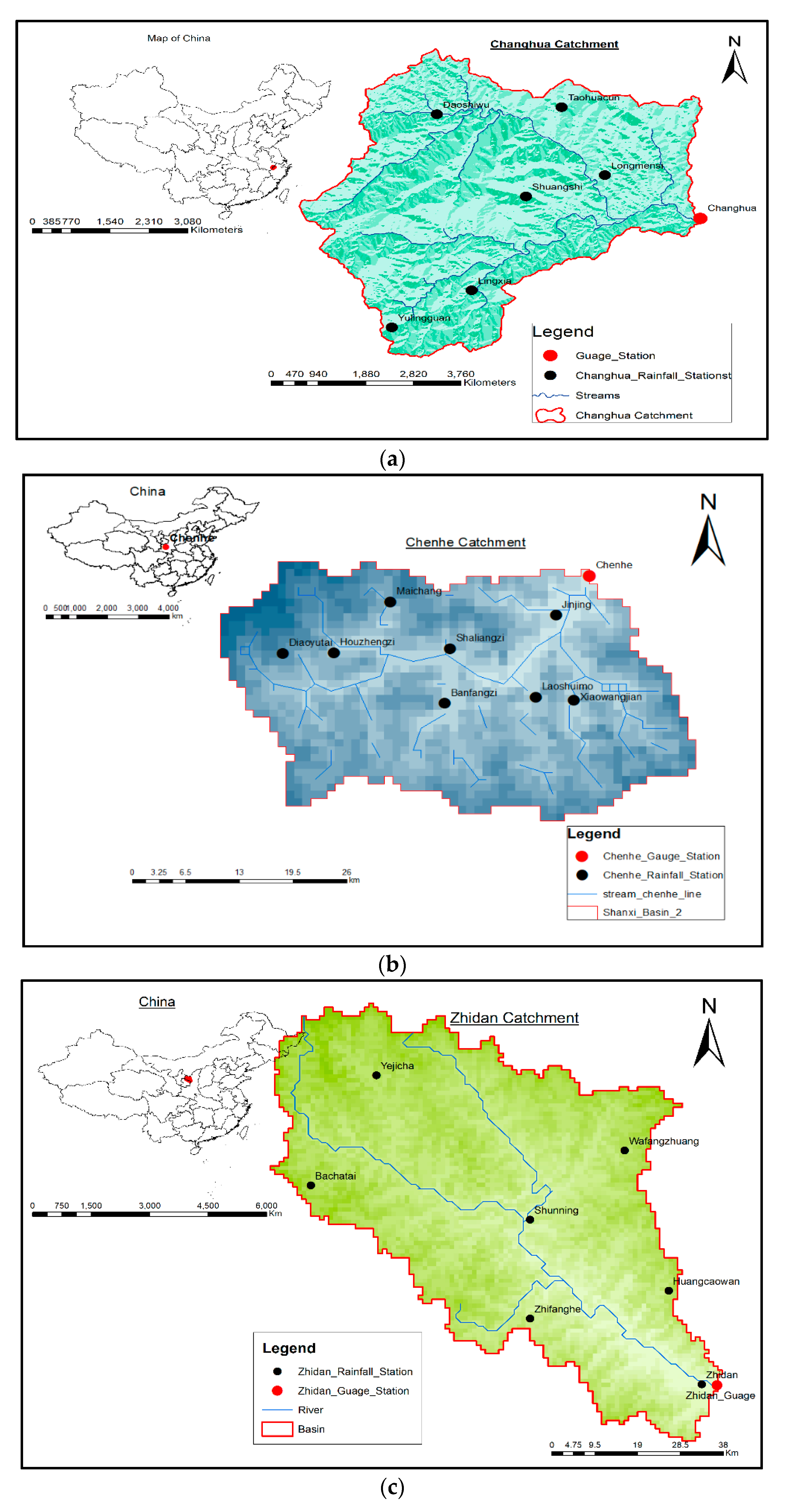
In this study, three different catchments in China were selected to evaluate the performance of ε-SVM and ANN, namely, the Changhua, Chenhe and Zhidan catchments, in humid, semi-humid and semi-arid regions, respectively. The total area of the Changhua river basin is 3442 km2, with a mainstream length of 1624 km, and an overall drop of 965 m. It is a subtropical monsoon climate with abundant rainfall and significant rainfall variation, with an annual rainfall of 1638.2 mm. During the spring season from March to early April, the southeasterly wind prevails upon the ground surface, and the amount of precipitation gradually increases. During the period from May to July, the frontal surface often stagnates or swings over the watershed, resulting in continuous rainfall with high rainfall intensity and long rainy seasons. During the summer months of July and September, the weather is hot, with prevailing southerly thunderstorm and typhoon rainfalls. From October to November, the weather is mainly sunny; from December to February, temperatures are low, with rain and snow weather.
Chenhe basin is located in the northern temperate zone, Shanxi province in China and belongs to the continental monsoon climate. The annual average precipitation is 700–900 mm. The local rainstorm is the primary cause of the flood. The average runoff depth is 100–500 mm, and the runoff coefficient is 0.2–0.5. It is a relatively high runoff yield area, with an erosion modulus of 100–200 t/km2.
Zhidan hydrologic station is located in Chengguan Town, Zhidan County, Shaanxi province, China. It is in the longitude of 108°46′ E, 36°49′ N. The topographic distribution of the upper reaches is comprised of high mountains, gorges, and barren beaches, with substantial slope changes, sparse vegetation, and severe soil erosion. The station catchment area is 744 km2, the river length is 81.3 km, and the distance from the estuary is 31 km. The regional climate features a moderate temperate semi-humid semi-arid zone, which is cold and dry in winter, and dry and windy in spring, with droughts and floods in summer, and which is cool and humid in autumn. The average annual temperature, precipitation, sediment transport, and discharge are 7.8 °C, 509.8 mm, 102 million tons, and 2610 m3/s, respectively. Floods are caused by heavy rains, with rapid fluctuations, sharp peaks, and short duration. The relationship between water level and discharge is generally poor.
This study used seven rainfall stations and one hydrological station for the Changhua catchment (Figure 1a) and eleven flood events between 07/04/1998 and 24/06/2002, nine rainfall stations and one hydrological station for the Changhua catchment (Figure 1b) and eleven flood events between 26/09/2003 and 30/09/2012, and seven rainfall stations and one hydrological station for the Zhidan catchment (Figure 1c) and fifteen flood events for the period between 27/07/2000 and 13/08/2010 for the development of the hydrological models using hourly data.
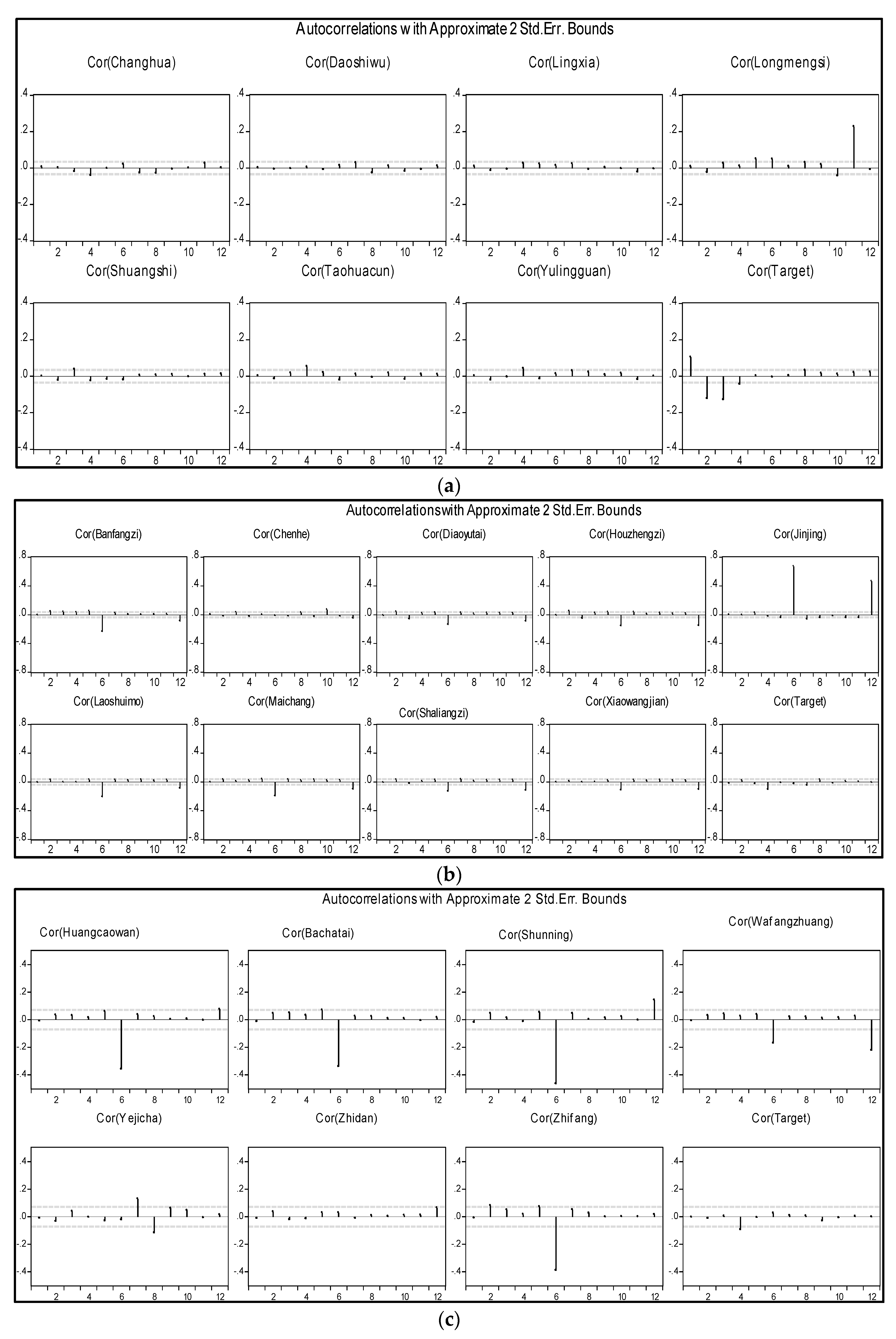
This research applied the vector autoregressive (VAR) method to determine the correlation over time and periodicities in the time series. VAR is one of the most useful, flexible, and easy-to-use models for analyzing the dynamic input of random disturbances on a system of variables [55]; Ref. [56] used VAR for streamflow sequence analysis. Ref [57] analyzed rainfall and groundwater level using VAR, and the results show that there is a significant influence of rainfall on groundwater level. Ref. [58] used VAR for rainfall forecasting; VAR accurately detected the correlation between rainfall and the coordinates of the isohyets; VAR successfully forecasted rainfall, and even outperformed the ARIMA model. Ref. [59] used monthly rainfall and streamflow data to develop streamflow trends using rainfall variability and determined causality between streamflow and rainfall for forecasting. Equation (13) shows a basic VAR model.
where is the K × 1 vector of the observable endogenous variables, is a d × 1 vector of the endogenous variables, are K × K matrices of lag coefficients to be estimated, C is a matrix of the exogenous variable coefficient to be estimated, is white noise. Different criteria are used for optimal lag selection, including the Akaike Information Criterion (AIC), the Schwarz Information Criterion (SC), and the Hannan-Quinn information criterion (HQ). This research adopted the SC criterion for selecting the optimal lag time of each variable, and the auto correlation function is plotted to show the significant lags in the time series of each variable.
Parameter optimization of the model plays a crucial role in the performance of the model. For the ANN model, learning rate, momentum value, and above all the network architecture were optimized using the logistic function and linear function as the activation function and output function, respectively. The optimized parameters for ε-SVM are the cost constant C and error tolerance (), and parameter ε controls the width of the e-insensitive loss function. Large ε-values result in a flatter estimated regression function. Parameter σ controls the RBF width, which reflects the distribution range of -values of training data. Parameters have commonly been determined by a trial and error process, which is inefficient and makes it difficult to achieve a favorable set of parameters that will provide a better-performing model—usually by means a costly grid search, which scales exponentially with the number of parameters used for finding optimal hyperparameters. Nonetheless, for effective optimization of parameters, the model should be nested with an automated, efficient optimization strategy for hyperparameters. Fortunately, the availability of advanced metaheuristic algorithms helps in providing the best solution for the multi-objective optimization problem.
This research adopted the ε-SVM and ANN models. SVM was trained by the RBF kernel function to transform a nonlinear problem into a linear function by mapping the input data into a hypothetical, high-dimensional feature space, while the back-propagation algorithm trained the ANN model. The data was standardized by the two models to remove periodicities present in the time series, and was divided into two datasets—training data set and testing data set—in a ratio of 68% and 32%, respectively. The windowing operator transformed the series data into features that describe the history for the current time point by taking a cross-section of data in time, followed by the application of a sliding window validation operator on the windowed data with a nested model algorithm inside for training and backtesting the hypothesis. When the model was finally developed, the model parameters, including (C, σ, ɛ for SVM) for SVM, (ε, α, network architecture) for ANN and cross-section, training size, and testing size, were finally optimized, and the model was set for streamflow prediction.
The performance of the models developed in this study was evaluated using seven different statistically different statistical measures of performance:
Root Mean Square Error (RMSE) measures overall performance across the entire range of the dataset. It is sensitive to small differences in the model performance and, being a squared measure, exhibits marked sensitivities to the larger errors that occur at higher magnitudes
Coefficient of determination (R2) describes the proportion of the total statistical variance in the observed dataset that can be explained by the model.
Nash Sutcliffe Efficiency (NSE) coefficient is sensitive to extreme values and might yield sub-optimal results when the dataset contains large outliers. Furthermore, it quantitatively describes the accuracy of model outputs other than the discharge.
Mean Square Relative Error (MSRE) provides a relative measure of model performance, the use of squared values makes it far more sensitive to the larger relative errors that will occur at lower magnitudes. It will, in consequence, be less critical of the larger absolute errors that tend to occur at higher magnitudes and more prone to potential fouling by small numbers in the observed record.
Mean Relative Error (MRE) is a relative metric that is sensitive to the forecasting errors that occur in the lower magnitudes of each dataset. In this case, because the errors are not squared, the evaluation metric is less sensitive to the larger errors that usually occur at higher values.
Mean Absolute Error (MAE) provides no information about underestimation or overestimation. It is not weighted towards higher-magnitude or lower-magnitude events, but instead evaluates all deviations from the observed values, in an equal manner and regardless of sign.
Mean Absolute Percentage Error (MAPE) is a relative metric that is sensitive to the forecasting errors that occur in the lower magnitudes of each dataset. In this case, because the errors are not squared, the evaluation metric is less sensitive to the larger errors that usually occur at higher magnitudes. It is nevertheless subject to potential “fouling” by small numbers in the observed record.
6. Results
Figure 2 shows the internal correlation within the time series of rainfall and streamflow data for humid, semi-humid, and semi-arid areas with a 5% level of confidence for a lag time of up to 12 h. Figure 2 indicates that the time series of a humid area is mostly stationary, with significant spikes in the streamflow data and rainfall data collected from Longmengsi station. The semi-humid area data has a few periodic events, noticed later in every rainfall time series, but the majority of the time series is stationary, whereas in semi-arid areas, the time series shows seasonality and there is a significant contribution to the variance in the time series from the many significant spikes showing periodicity within the time series. Table 1 indicates that there are shorter delays (2–4 h) in the time series of humid areas, and longer delays (7–8 h) in semi-humid and semi-arid areas.
Selection of significant input variables is an essential step in the development of time series forecasting models to improve the performance of the model by removing irrelevant and redundant variables that add extra noise, which reduces the accuracy and speed of the model [60]. Correlated input variables affect the prediction ability of the model, because they obscure the true relationship that exists between important variables [61]. This study adopted a model-based approach by using a brute force feature selection method to select the significant input variables, trying all possible combinations of attribute selection in an automatic search process that optimized some indicators for model performance. Since models respond differently to input variables, SVM and ANN operate as a subprocess and return a performance vector; then, the brute force operator selects the feature set with the best performance vector Table 2.
7. Discussion
Table 3 shows seven statistical measures of performance used to assess the performance of the models for the three catchments. One distinct feature is that the models performed phenomenally during the simulation process of all the catchments. SVM successfully simulated streamflow better than ANN, as indicated by all metrics in Table 3. According to R2 and NSE, both models accurately predicted the maximum flow for humid and semi-humid regions. However, the value of AME shows that ANN underestimated the minimum streamflow of the humid area. SVM successfully simulated streamflow of the semi-arid area, while ANN poorly simulated the both minimum and maximum flows of the streamflow, as indicated by R2, NSE, MSRE, and MRE. The results tie in well with those of [22,62]. Due to the high degree of spatial and temporal variability in semi-arid areas, ANN underperformed, because ANN often fails to find global optima in complex and high-dimensional parameter spaces [63].
For the forecasted time in humid areas, SVM successfully forecasted streamflow up to 4 h lead time, and ANN forecasted up to 5 h, according to R2 and NSE values. This indicated that the models predicted the streamflow very well, though ANN overestimated the low flow events according to MSRE and MAE, signifying a high deviation of predicted values from the observed values. This result is in agreement with those of [22,64], in which the authors compared the performances of ANN and SVM for streamflow forecasting. From Table 3, in the semi-humid area, the ANN model obtained the highest R2 and NSE values for all of the forecasted period, and also obtained a lower RMSE for all periods than the SVM model. However, SVM performed well when using other evaluation metrics.
Regarding relative evaluation metrics such as MRE, MSRE and MAE, ANN did not perform well, for 1 h and 3 h forecast time, especially, the ANN model underestimated the minimum flow, as indicated by the MRE values, which were −0.06 and −0.13, respectively. ANN was applied for hydrological modeling, the author emphasized that ANN models in hydrology tend to perform very well according to statistical metrics sensitive to errors occurring at higher magnitudes (R2, NSE, RMSE), but perform poorly when estimating low flows because of relative metrics, which are more critical for errors occurring in the lower magnitudes (MRE, MAPE, MSRE) [65]. Ref. [65] used integrated GA to overcome the ANN problem of failing to estimate minimum flows, and also to improve the overall performance of ANN in streamflow simulation. As for semi-arid catchments, both models failed to forecast streamflow, with only the SVM model closely predicting streamflow in the results for the 1-hour-ahead prediction, as indicated by R2, RMSE, MAE, MAPE and MRE. All metrics critically penalize ANN for 1 h lead time. SVM is penalized more by R2 than ANN as forecasting time increases, whereas MSRE and NSE severely penalize both models with increasing lead times. Regular ANN was compared with wavelet-ANN (WA-ANN) for 1–3-day lead time forecasting, and as indicated by R2, ANN and WA-ANN obtained 0.62 and 0.78 for a 1 day lead time, and 0.4 and 0.42 for a 3 day lead time, respectively. These results are in agreement with the findings of this paper regarding the decreasing value of R2 obtained with increasing lead times [66]. NSE is used to assess the predictive power of hydrological models. The threshold values indicating a model’s degree of sufficiency are suggested to be between 0.5 < NSE < 0.65. Therefore, the models performed poorly on semi-arid catchments, and only predicted the one-hour lead time, which is still not satisfactory.
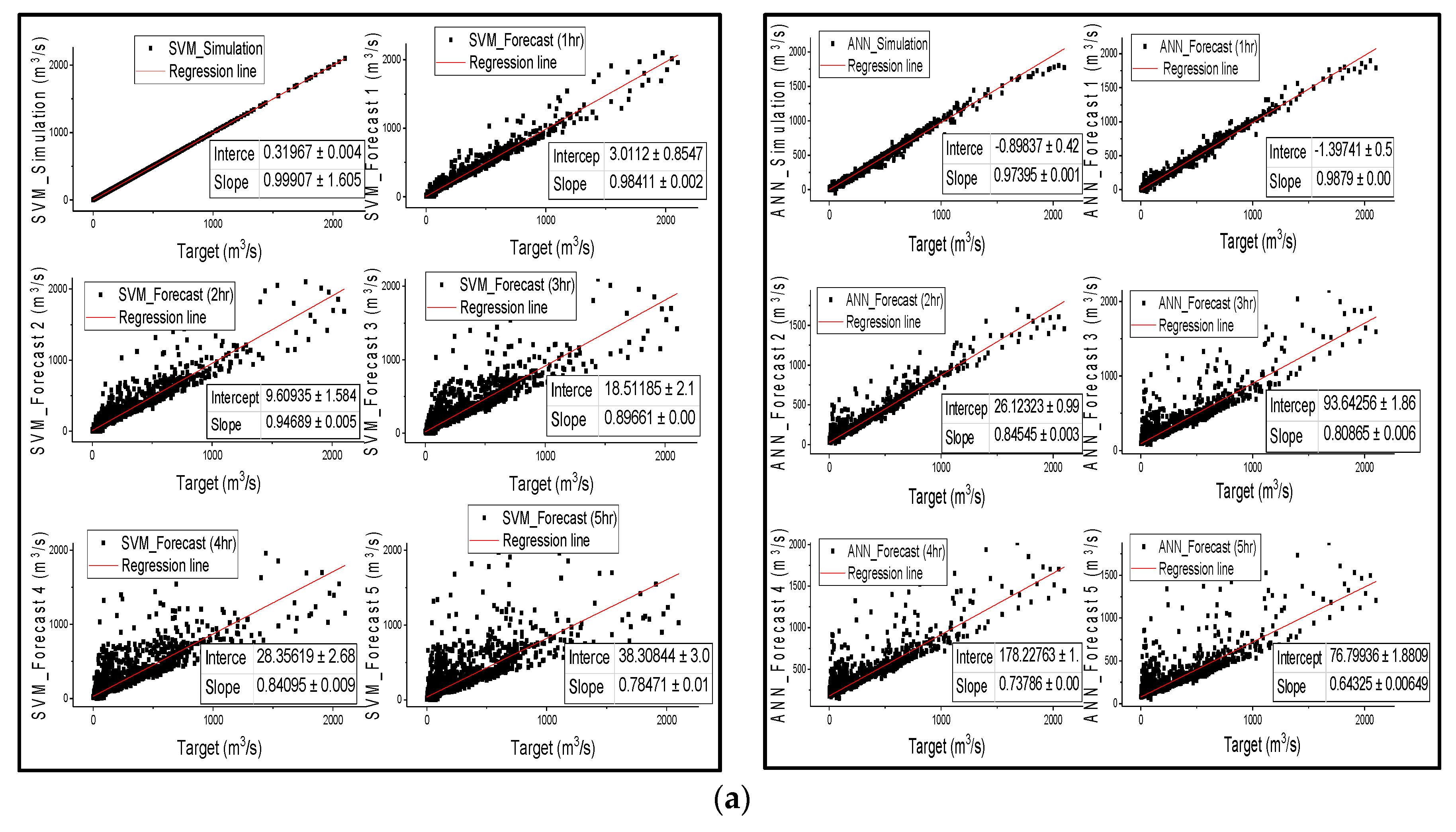
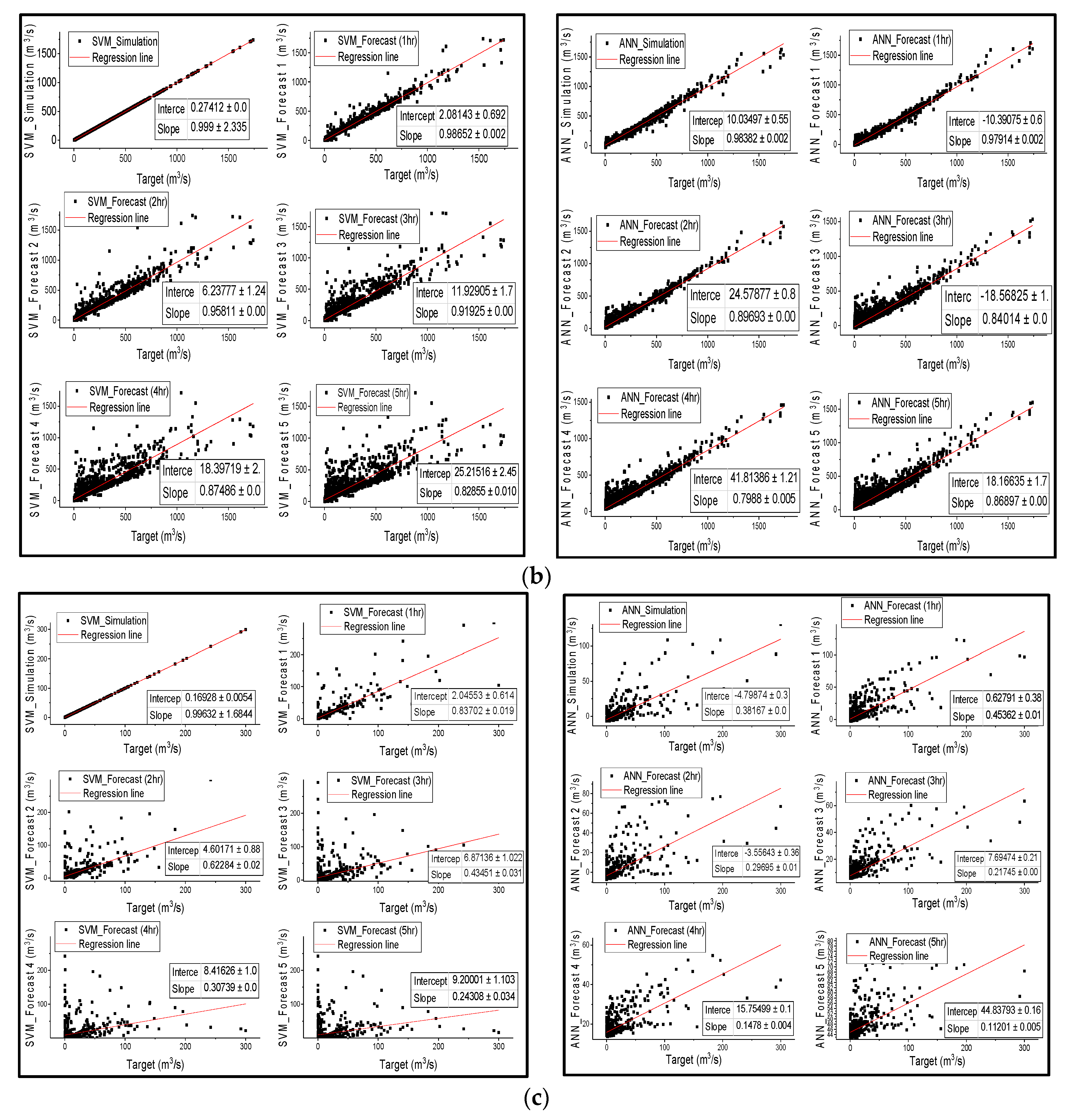
The results from Figure 3 are in agreement with the results in Table 3, that SVM outperformed ANN in streamflow simulation of all catchments; nonetheless, both models successfully simulated streamflow, except for ANN in semi-arid areas, as confirmed by all metric values in Table 3. Points are distributed along the regression line during the first 3 h of lead time for the SVM and ANN models in humid and semi-humid areas, and then spread wide from the line of perfect agreement as the lead time increases. However, the wide distribution of points from the regression line is more significantly noticeable in SVM than in ANN. The notable feature is that the correlation coefficient between the observed discharge and the forecasted discharge also diminishes with the increase in forecast time; Figure 3 is in agreement with Table 3 that the linear regression relationship behavior between observed and estimated streamflow shows that the performance of the models decreases from humid regions to drier regions.
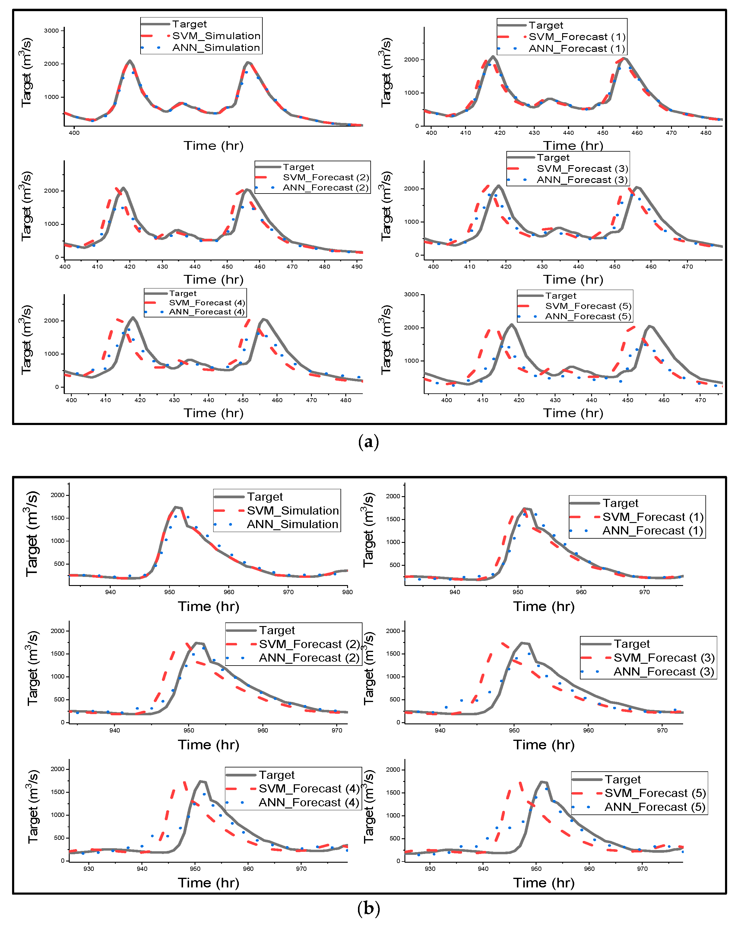
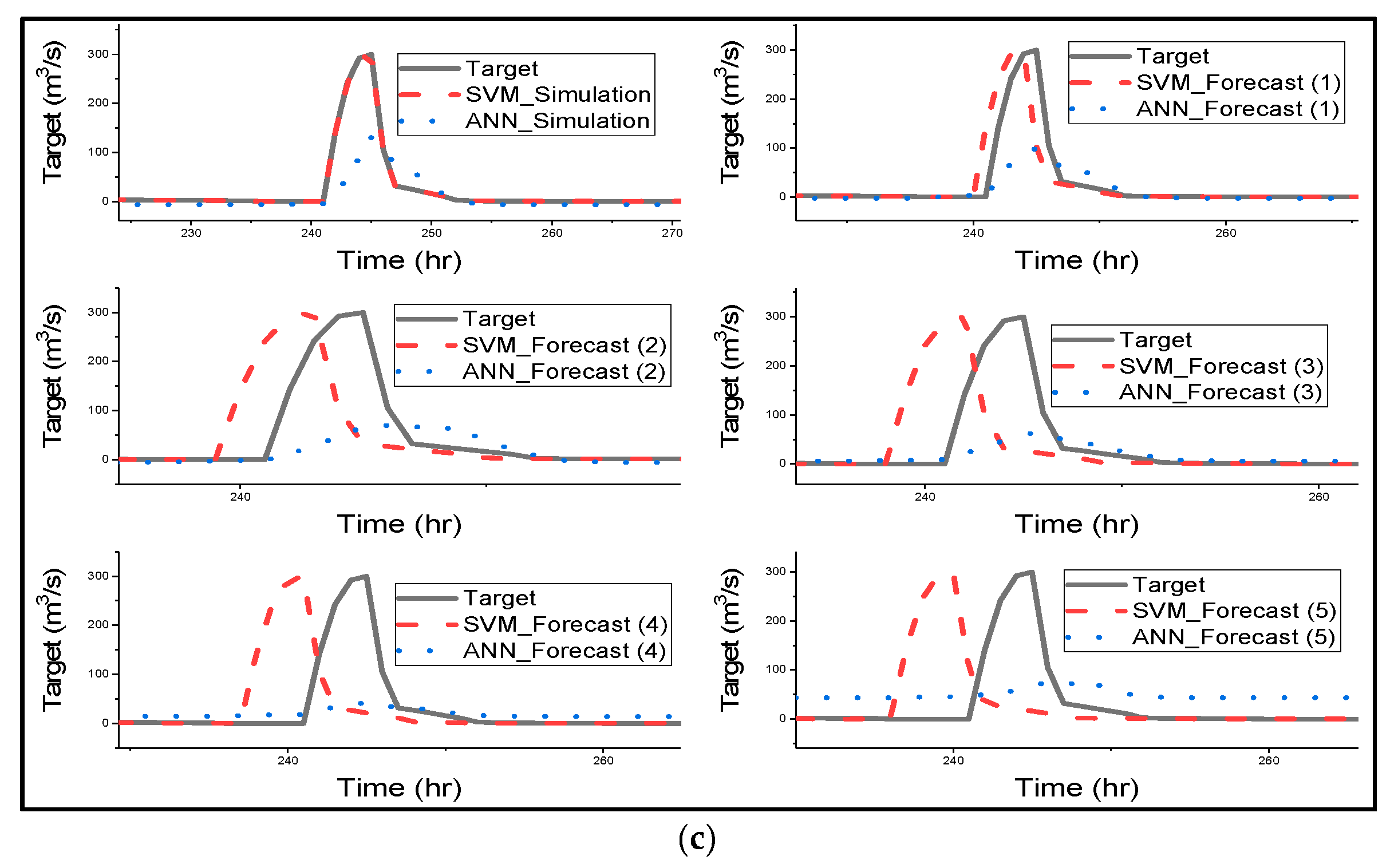
Figure 4 gives a clear graphical representation of how the ANN and SVM model has simulated, and forecasted streamflow for all different catchments [67] stated that SVM could be able to prevent the influence of non-SV over the model during training by optimizing SV, and [68] mentioned that SVMs are suitable for nonlinear regression than ANN as they can identify optimal global solution. The SVM model managed to predict the shape of the hydrograph very well for simulation and all forecasted results. Most importantly SVM successfully predicted the lows and peaks of the time series of all catchments. Furthermore, SVM accurately simulated the streamflow of all catchments as indicated in Table 3 and Figure 3. SVM was used for streamflow forecasting, and the model accurately simulated the streamflow of Lang Yang river basin [16]. ANN model also performed very well in humid and semi-humid catchments. Figure 4 clearly shows that SVM outperformed ANN in streamflow simulation of all catchments.
The notable performance from Figure 4 is that as forecast time increases, there is an increase in the lag phase between the predicted hydrograph by SVM and the observed hydrograph. The lag is noticeable in the forecasted period of 3 h of Changhua streamflow and increases as forecast time increases. Meanwhile, in the Chenhe catchments, the lag is noticeable within 3 h forecast time. Lastly, for Zhidan, the streamflow in Figure 4 is in agreement with the scatter plots for the performance of the model, as the lag is visible at 1 h lead time. Figure 4 explains the results in Table 3, indicating that all of the metrics that measure overall performance are more sensitive to hydrograph lags than the peaks, and also removes the impression given by Figure 3 that SVM overestimated the maximum flows, as this is due to the lags in the predicted hydrographs. Ref. [69] used SVR for flood stage forecasting, and the model successfully forecasted flood stage, although the results were slightly weaker than the simulation results. SVR effectively forecasted the flood stage with 1 h to 6 h lead time, and the time lag is visible for 5 h to 6 h lead times, but the phase lag is insignificant when compared to the SVM results in this study. The authors suggest that the phase lags could be due to the sensitivity of the model with respect to the lag of the input variables.
Figure 4 shows that ANN forecasted streamflow very well for humid and semi-humid catchments, but the model slightly underestimated the peak flows, and there was a drop in estimated peak flows as forecast time increased; a significant decline in estimated peak is visible with a 5 h lead time. Furthermore, the noticeable characteristic of ANN is that as the lead time increases, the model fails to predict the trend or shape of the observed time series, especially the lower and moderate flows. [65] applied ANN for streamflow forecasting, and the results are quite similar to the results of this study. The authors trained ANN using BP and GA, and the results indicate that ANN models trained with the BP algorithm tend to overestimate the minimum streamflow; therefore, Srinivasule and Jain applied GA to solve the problem. However, the ANN model trained with BP also overestimated the peak flows, whereas in this study, ANN has the problem of underestimating the peak flows. Finally, the ANN model failed to forecast semi-arid streamflow; the model completely underestimated the peak of the hydrograph for all forecasted times. This could be due to the effect of low rainfall being overestimated by the model [63].
This study applied different metrics that are critical to errors occurring at low and at peak flow, as well as those that measure the overall performance of the model. This illustrates that every statistical index has its weaknesses and limitations, as observed in Table 3, in which NSE, R2, and RMSE heavily penalized SVM, but not MSRE, MRE and MAPE; while metrics like MAE, MSRE, MRE, and MAPE punished ANN more heavily than overall measures of performance. Therefore, consideration of other analysis tools such as graphical representation is prudent before accepting or rejecting a model based on the values of the metrics without acknowledging the flaws.
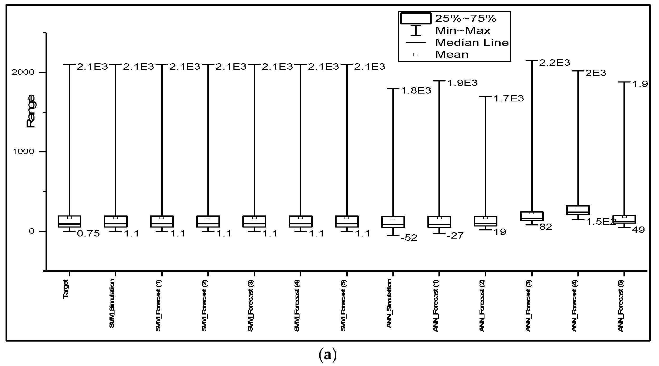
Figure 5 was considered for further analysis in the performance of the ɛ-SVM and ANN models. The box plots were formed by determining the median of the data set, then the median in the lower and upper quartiles of the data set, and finally the lower and upper extremes of the data set, which are connected by the whisker to the box showing the minimum and the maximum of the data set. Figure 5 shows that the SVM model accurately predicted the observed time series of all catchments, as the predicted results have the same mean, median, minimum and interquartile range. SVM slightly overestimated the peak flows with 4 h and 5 h lead times for humid areas, whereas ANN underestimated the peaks with 1–3 h lead times, and with 3–5 h lead times, the performance of the model declined, as the mean, median and range were significantly different from the observed data. Furthermore, the model overestimated the minimum flows, as indicated in Table 3. Figure 5c clearly shows that the results predicted by SVM are similar to the observed values. This confirms that for semi-arid catchments, the metrics were sensitive to the lags of the predicted hydrographs. Meanwhile, ANN did not perform well in semi-arid regions; the nonlinearity and variability of the basin could have affected the prediction accuracy of the model, because of overparameterization effects and the optimization algorithm failing to reach global optima in complex and high-dimensional spaces [63]. Figure 5 clearly shows that SVM simulated and forecasted the streamflow of all catchments better than ANN. SVM and ANN were applied for streamflow forecasting, and their results concur with the results of this study, indicating that both models performed well in predictions of streamflow, especially in the humid and semi-humid areas [26,64,70]. The results of this study are in agreement with the results of other studies, suggesting that SVM performs better than ANN. This is because SVMs are capable of evaluating more relevant information conveniently [71]. Furthermore, its quality of abiding by a structural risk minimization principle helps SVM to maximize the margin; thus, its generalizability does not decrease [44].
8. Conclusions
This study developed ANN and SVM models for flood simulation and forecasting in humid, semi-humid and semi-arid catchments using input antecedent hourly rainfall date and output antecedent hourly streamflow data. Then, the Brute force method was applied for the selection of the significant input variables of every model, and the ES algorithm was employed for the optimization of model parameters. The models were compared for a 1–5 h lead time for all catchments. The results showed that the ANN model successfully established accurate and reliable streamflow forecasting of humid and semi-humid catchments, although the model had the problem of underestimating the peak flow. Meanwhile, the SVM model successfully simulated and forecasted the streamflow of all basins, and the SVM model was able to maintain excellent accuracy for the minimum and maximum values of all basins and forecast times. The only significant drawback affecting the prediction accuracy of SVM was the presence of lags, and the lag phase increased with the forecast lead time.
Performance of SVM could be improved by removing the lags in the forecasted time series, especially of semi-arid areas, because lags were observed in 1 h lead time predictions in comparison to other areas. Although delays are inevitable when forecasting time series, ANN was found to be efficient in the elimination of lags. However, ANN performed poorly in semi-arid areas, as it overestimated minimum flow and underestimated peak flows. The possible reason for which ANN and SVM performed well in humid and semi-arid areas could be that the rainfall-runoff relationship is not complicated or dynamic, because water storage is near saturation. Whereas, in semi-arid areas, the performance is poor because of the complex and dynamic rainfall-relationship. To improve the performance of the ANN and SVM models in forecasting the streamflow of semi-arid areas, other methods for determining significant input variables should be exploited, such as evolutionary algorithms, or additional model parameter optimization. The ensemble of the models could also help to improve prediction and eliminate the lags in the forecasted time series.
Author Contributions
T.M.B.: Designed, developed the models, and the conceptual framework and analysed the data, wrote the manuscript; Z.L.: Devised and supervised the project, and the findings of this work, verfified analytical methods. All authors discussed the results and contributed to the final manuscript.
Funding
This research was supported by Natural Science Foundation of China (51679061), National Key R&D Program of China (Grant No. 2016YFC0402705) and by the Research Funds for the Central Universities 2018B11014.
Acknowledgments
First of all I would like to deeply thank Almighty God for granting me good health, strength, and knowledge to undertake this research study and complete it soon enough. I woud also like to thank my supervisor Prof Zhijia Li for his exceptional support, guidance, and supervision throughout this research. I exprss my gratitude to Wembu Huo for helping with data collection and his support. Lastly I would like to immensely thank my family and friends for their breathtaking love, support, motivation and encouragement at all times ensuring that the fire keeps burning.
Conflicts of Interest
Authors declare no conflicts of interest.
References
- Solomatine, D.P. Data-Driven Modeling and Computational Intelligence Methods in Hydrology. In Encyclopedia of Hydrological Sciences; John Wiley & Sons, Ltd.: Chichester, UK, 2005. [Google Scholar] [CrossRef]
- Solomatine, D.P.; Ostfeld, A. Data-driven modelling: Some past experiences and new approaches. J. Hydroinform. 2008, 10, 3. [Google Scholar] [CrossRef]
- Solomatine, D.P.; Price, R.K. Innovative approaches to flood forecasting using data driven and hybrid modelling. Education 2004, 1–8. [Google Scholar] [CrossRef]
- Anderson, M.; McDonnell, J. Encyclopedia of Hydrological Sciences. 2005. Available online: http://www.citeulike.org/group/1428/article/764778 (accessed on 28 July 2018).
- Mosavi, A.; Ozturk, P. Flood Prediction Using Machine Learning, Literature Review. Water 2018, 10, 1536. [Google Scholar] [CrossRef]
- Jin, H.; Liang, R.; Wang, Y.; Tumula, P. Flood-runoff in semi-arid and sub-humid regions, a case study: A simulation of Jianghe watershed in northern China. Water 2015, 7, 5155–5172. [Google Scholar] [CrossRef]
- Kan, G.; He, X.; Ding, L.; Li, J.; Liang, K.; Hong, Y. Study on applicability of conceptual hydrological models for flood forecasting in humid, semi-humid semi-arid and arid basins in China. Water 2017, 9. [Google Scholar] [CrossRef]
- Wang, L.; Li, Z.; Bao, H. Application of developed grid-ga distributed hydrologic model in semi-humid and semi-arid basin. Trans. Tianjin Univ. 2010, 16, 209–215. [Google Scholar] [CrossRef]
- Pilgrim, D.H.; Chapman, T.G.; Doran, D.G. Problems of rainfall-runoff modelling in arid and semiarid regions. Hydrol. Sci. J. 1988, 33, 379–400. [Google Scholar] [CrossRef] [Green Version]
- Hao, G.; Li, J.; Song, L.; Li, H.; Li, Z. Comparison between the TOPMODEL and the Xin’anjiang model and their application to rainfall runoff simulation in semi-humid regions. Environ. Earth Sci. 2018, 77. [Google Scholar] [CrossRef]
- Lin, X. Flash Floods in Arid and Semi-Arid Zones. International Hydrological Programme—UNESCO. 1999. Available online: http://bases.bireme.br/cgi-bin/wxislind.exe/iah/online/?IsisScript=iah/iah.xis&src=google&base=REPIDISCA&lang=p&nextAction=lnk&exprSearch=92304&indexSearch=ID (accessed on 20 October 2018).
- Dunne, T.; Black, R.D. Partial Area Contributions to Storm Runoff in a Small New England Watershed. Water Resour. Res. 1970, 6, 1296–1311. [Google Scholar] [CrossRef]
- Marchi, L.; Borga, M.; Preciso, E.; Gaume, E. Characterisation of selected extreme flash floods in Europe and implications for flood risk management. J. Hydrol. 2010, 394, 118–133. [Google Scholar] [CrossRef]
- Ragettli, S.; Zhou, J.; Wang, H.; Liu, C.; Guo, L. Modeling flash floods in ungauged mountain catchments of China: A decision tree learning approach for parameter regionalization. J. Hydrol. 2017, 555, 330–346. [Google Scholar] [CrossRef]
- Huo, W.; Li, Z.; Wang, J.; Yao, C.; Zhang, K.; Huang, Y. Multiple hydrological models comparison and an improved Bayesian model averaging approach for ensemble prediction over semi-humid regions. Stoch. Environ. Res. Risk Assess. 2018. [Google Scholar] [CrossRef]
- Yu, P.S.; Chen, S.T.; Chang, I.F. Support vector regression for real-time flood stage forecasting. J. Hydrol. 2006. [Google Scholar] [CrossRef]
- Li, X.-L.; Lü, H.; Horton, R.; An, T.; Yu, Z. Real-time flood forecast using the coupling support vector machine and data assimilation method. J. Hydroinform. 2014, 16, 973. [Google Scholar] [CrossRef]
- Dibike, Y.B.; Velickov, S.; Solomatine, D.; Abbott, M.B. Model induction with support vector machines: Introduction and applications. J. Comput. Civ. Eng. 2001, 15, 208–216. [Google Scholar] [CrossRef]
- Tongal, H.; Booij, M.J. Simulation and forecasting of streamflows using machine learning models coupled with base flow separation. J. Hydrol. 2018, 564, 266–282. [Google Scholar] [CrossRef]
- Adnan, R.M.; Yuan, X.; Kisi, O.; Adnan, M.; Mehmood, A. Stream Flow Forecasting of Poorly Gauged Mountainous Watershed by Least Square Support Vector Machine, Fuzzy Genetic Algorithm and M5 Model Tree Using Climatic Data from Nearby Station. Water Resour. 2018, 32, 4469–4486. [Google Scholar] [CrossRef]
- Sharifi Garmdareh, E.; Vafakhah, M.; Eslamian, S.S. Regional flood frequency analysis using support vector regression in arid and semi-arid regions of Iran. Hydrol. Sci. J. 2018, 63, 426–440. [Google Scholar] [CrossRef]
- Adnan, R.; Yuan, X.; Kisi, O.; Yuan, Y. streamflow forecasting using artificial neural network and support vector machine model. Am. Sci. Res. J. Eng. Technol. Sci. 2017, 29, 286–294. [Google Scholar] [CrossRef]
- Yu, P.-S.; Yang, T.-C.; Chen, S.-Y.; Kuo, C.-M.; Tseng, H.-W. Comparison of random forests and support vector machine for real-time radar-derived rainfall forecasting. J. Hydrol. 2017, 552, 92–104. [Google Scholar] [CrossRef]
- Su, J.; Wang, X.; Liang, Y.; Chen, B. GA-Based Support Vector Machine Model for the Prediction of Monthly Reservoir Storage. J. Hydrol. Eng. 2014, 19, 1430–1437. [Google Scholar] [CrossRef]
- Yin, Z.; Wen, X.; Feng, Q.; He, Z.; Zou, S.; Yang, L. Integrating genetic algorithm and support vector machine for modeling daily reference evapotranspiration in a semi-arid mountain area. Hydrol. Res. 2017, 48, 1177–1191. [Google Scholar] [CrossRef]
- Aichouri, I.; Hani, A.; Bougherira, N.; Djabri, L.; Chaffai, H.; Lallahem, S. River Flow Model Using Artificial Neural Networks. Energy Procedia 2015, 74, 1007–1014. [Google Scholar] [CrossRef] [Green Version]
- Dounia, M.; Sabri, D.; Yassine, D. Rainfall—Rain off Modeling Using Artificial Neural Network. APCBEE Procedia 2014, 10, 251–256. [Google Scholar] [CrossRef]
- He, Z.; Wen, X.; Liu, H.; Du, J. A comparative study of artificial neural network, adaptive neuro fuzzy inference system and support vector machine for forecasting river flow in the semiarid mountain region. J. Hydrol. 2014. [Google Scholar] [CrossRef]
- Raghavendra, S.; Deka, P.C. Support vector machine applications in the field of hydrology: A review. Appl. Soft Comput. J. 2014. [Google Scholar] [CrossRef]
- Perera, E.D.P.; Lahat, L. Fuzzy logic based flood forecasting model for the Kelantan River basin, Malaysia. J. Hydro-Environ. Res. 2015. [Google Scholar] [CrossRef]
- El-Shafie, A.; Taha, M.R.; Noureldin, A. A neuro-fuzzy model for inflow forecasting of the Nile river at Aswan high dam. Water Resour. Manag. 2007. [Google Scholar] [CrossRef]
- Mukerji, A.; Chatterjee, C.; Raghuwanshi, N.S. Flood Forecasting Using ANN, Neuro-Fuzzy, and Neuro-GA Models. J. Hydrol. Eng. 2009. [Google Scholar] [CrossRef]
- Al-Abadi, A.M. Modeling of stage–discharge relationship for Gharraf River, southern Iraq using backpropagation artificial neural networks, M5 decision trees, and Takagi–Sugeno inference system technique: A comparative study. Appl. Water Sci. 2016, 6, 407–420. [Google Scholar] [CrossRef]
- Khan, M.Y.A.; Hasan, F.; Panwar, S.; Chakrapani, G.J. Neural network model for discharge and water-level prediction for Ramganga River catchment of Ganga Basin, India. Hydrol. Sci. J. 2016, 61, 2084–2095. [Google Scholar] [CrossRef]
- Wang, L.; Zeng, Y.; Chen, T. Back propagation neural network with adaptive differential evolution algorithm for time series forecasting. Expert Syst. Appl. 2015, 42, 855–863. [Google Scholar] [CrossRef]
- Veintimilla-Reyes, J.; Cisneros, F.; Vanegas, P. Artificial Neural Networks Applied to Flow Prediction: A Use Case for the Tomebamba River. Procedia Eng. 2016, 162, 153–161. [Google Scholar] [CrossRef] [Green Version]
- Nourani, V. An Emotional ANN (EANN) approach to modeling rainfall-runoff process. J. Hydrol. 2017, 544, 267–277. [Google Scholar] [CrossRef]
- Kişi, Ö. River flow forecasting and estimation using different artificial neural network techniques. Hydrol. Res. 2008, 39, 27–40. [Google Scholar] [CrossRef]
- Campolo, M.; Soldati, A.; Andreussi, P. Artificial neural network approach to flood forecasting in the River Arno. Hydrol. Sci. J. 2003, 48, 381–398. [Google Scholar] [CrossRef] [Green Version]
- Jayawardena, A.W.; Fernando, T. River flow prediction: An artificial neural network approach. In Regional Management of Water Resources; Iahs Publication: Wallingford, UK, 2001; pp. 239–246. [Google Scholar]
- Boser, J.A. Microcomputer Needs Assessment of American Evaluation Association Members. Am. J. Eval. 1992, 13, 92–93. [Google Scholar] [CrossRef]
- Vapnik, V. The Support Vector Method of Function Estimation. In Nonlinear Modeling; Springer: Boston, MA, USA, 1998; pp. 55–85. [Google Scholar] [CrossRef]
- Wu, M.C.; Lin, G.F. An hourly streamflow forecasting model coupled with an enforced learning strategy. Water 2015, 7, 5876–5895. [Google Scholar] [CrossRef]
- Smola, A. Regression Estimation with Support Vector Learning Machines. Master’s Thesis, Technische Universitat Munchen, Munich, Germany, 1996; pp. 1–78. [Google Scholar] [CrossRef]
- Wang, W.; Xu, D.; Chau, K.; Chen, S. Improved annual rainfall-runoff forecasting using PSO–SVM model based on EEMD. J. Hydroinform. 2013, 15, 1377–1390. [Google Scholar] [CrossRef]
- Thissen, U.; van Brakel, R.; de Weijer, A.; Melssen, W.; Buydens, L.M. Using support vector machines for time series prediction. Chemometr. Intell. Lab. Syst. 2003, 69, 35–49. [Google Scholar] [CrossRef]
- Simon, D. Evolutionary Optimization Algorithms; John Wiley & Sons: Hoboken, NJ, USA, 2013. [Google Scholar] [CrossRef]
- Beyer, H.-G.; Schwefel, H.-P. Evolution strategies–A comprehensive introduction. Nat. Comput. 2002, 1, 3–52. [Google Scholar] [CrossRef]
- Costa, L.; Oliveira, P. Evolutionary algorithms approach to the solution of mixed integer non-linear programming problems. Comput. Chem. Eng. 2001, 25, 257–266. [Google Scholar] [CrossRef]
- Richter, J.N. On Mutation and Crossover in the Theory of Evolutionary Algorithms. ProQuest Dissertations and Theses. 2010. Available online: https://search.proquest.com/docview/305202204?accountid=11664 (accessed on 15 September 2018).
- Yin, X.; Zhang, J.; Wang, X. Sequential injection analysis system for the determination of arsenic by hydride generation atomic absorption spectrometry. Fenxi Huaxue. 2004, 32, 1365–1367. [Google Scholar] [CrossRef]
- Hansen, N.; Ostermeier, A. Completely Derandomized Self-Adaptation in Evolution Strategies. Evol. Comput. 2001, 9, 159–195. [Google Scholar] [CrossRef] [PubMed] [Green Version]
- Gholamipoor, M.; Ghadimi, P.; Alavidoost, M.H.; Feizi Chekab, M.A. Application of evolution strategy algorithm for optimization of a single-layer sound absorber. Cogent Eng. 2014, 1. [Google Scholar] [CrossRef]
- Chen, Z.; He, Y.; Chu, F.; Huang, J. Evolutionary strategy for classification problems and its application in fault diagnostics. Eng. Appl. Artif. Intell. 2003, 16, 31–38. [Google Scholar] [CrossRef]
- Zivot, E.; Wang, J. Vector Autoregressive Models for Multivariate Time Series. In Modeling Financial Time Series with S-PLUS®; Springer: Berlin, Germany, 2006; pp. 385–429. [Google Scholar] [CrossRef]
- Ledolter, J. The analysis of multivariate time series applied to problems in hydrology. J. Hydrol. 1978, 36, 327–352. [Google Scholar] [CrossRef]
- Hau, M.C.; Tong, H. A practical method for outlier detection in autoregressive time series modelling. Stoch. Hydrol. Hydraul. 1989, 3, 241–260. [Google Scholar] [CrossRef]
- Nugroho, A.; Hartati, S.; Mustofa, K. Vector Autoregression (Var) Model for Rainfall Forecast and Isohyet Mapping in Semarang–Central Java–Indonesia. J. Adv. Comput. Sci. Appl. 2014, 5, 44–49. [Google Scholar] [CrossRef]
- Iddrisu, W.A.; Nokoe, K.S.; Akoto, I. Modelling the trend of flows with respect to rainfall variability using vector autoregression. Int. J. Adv. Res. 2016, 4, 125–140. [Google Scholar] [CrossRef]
- Tran, H.D.; Muttil, N.; Perera, B.J.C. Selection of significant input variables for time series forecasting. Environ. Model. Softw. 2015, 64, 156–163. [Google Scholar] [CrossRef]
- Alexandridis, A.; Patrinos, P.; Sarimveis, H.; Tsekouras, G. A two-stage evolutionary algorithm for variable selection in the development of RBF neural network models. Chemometr. Intell. Lab. Syst. 2005, 75, 149–162. [Google Scholar] [CrossRef]
- Gizaw, M.S.; Gan, T.Y. Regional Flood Frequency Analysis using Support Vector Regression under historical and future climate. J. Hydrol. 2016, 538, 387–398. [Google Scholar] [CrossRef]
- De Vos, N.J.; Rientjes, T.H.M. Constraints of artificial neural networks for rainfall-runoff modelling: Trade-offs in hydrological state representation and model evaluation. Hydrol. Earth Syst. Sci. Discus. 2005, 2, 365–415. [Google Scholar] [CrossRef]
- Kalteh, A.M. Monthly river flow forecasting using artificial neural network and support vector regression models coupled with wavelet transform. Comput. Geosci. 2013, 54, 1–8. [Google Scholar] [CrossRef]
- Srinivasulu, S.; Jain, A. Rainfall-Runoff Modelling: Integrating Available Data and Modern Techniques. In Practical Hydroinformatics: Computational Intelligence and Technological Developments in Water Applications; Springer: Berlin/Heidelberg, Germany, 2008; pp. 59–70. [Google Scholar] [CrossRef]
- Adamowski, J.; Sun, K. Development of a coupled wavelet transform and neural network method for flow forecasting of non-perennial rivers in semi-arid watersheds. J. Hydrol. 2010, 390, 85–91. [Google Scholar] [CrossRef]
- Bhagwat, P.P.; Maity, R. Multistep-ahead River Flow Prediction using LS-SVR at Daily Scale. J. Water Resour. Prot. 2012, 4, 528–539. [Google Scholar] [CrossRef]
- Tehrany, M.S.; Pradhan, B.; Mansor, S.; Ahmad, N. Flood susceptibility assessment using GIS-based support vector machine model with different kernel types. Catena 2015, 125, 91–101. [Google Scholar] [CrossRef]
- Yu, P.S.; Chen, S.T.; Chang, I.F. Flood stage forecasting using support vector machines. Geophys. Res. Abstr. 2005, 7, 41–76. [Google Scholar]
- Suliman, A.; Nazri, N.; Othman, M.; Abdul, M.; Ku-mahamud, K.R. Artificial Neuaral Network and Support Vector Machine in Flood Forecasting: A Review. J. Hydroinform. 2013, 15, 327–332. [Google Scholar] [CrossRef]
- Cristianini, N.; Shawe-Taylor, J. An Introduction to Support Vector Machines and Other Kernel-Based Methods. 2000. Available online: https://books.google.com.br/books?hl=en&lr=&id=_PXJn_cxv0AC&oi=fnd&pg=PR9&dq=:+An+Introduction+to+Support+Vector+Machines+and+Other+Kernel-Based+Learning+Methods&ots=xSQi5BXq3e&sig=e0GieLD8UrBJf8Xf060CumoL0wA (accessed on 21 December 2018).
Figure 1.
(a) Changhua catchment, (b) Chenhe catchment, (c) Zhidan catchment.

Figure 2.
Autocorrelation plots of rainfall and streamflow for (a) Humid, (b) Semi-Humid, (c) Semi-arid catchments.
Figure 2.
Autocorrelation plots of rainfall and streamflow for (a) Humid, (b) Semi-Humid, (c) Semi-arid catchments.

Figure 3.
Scatter plots of the target (measure streamflow) versus simulated and forecasted streamflow from 1 h lead time to 5 h lead time for Changhua basin, Chenhe basin and Zhidan basin (a), (b) and (c) respectively for both SVM and ANN models.
Figure 3.
Scatter plots of the target (measure streamflow) versus simulated and forecasted streamflow from 1 h lead time to 5 h lead time for Changhua basin, Chenhe basin and Zhidan basin (a), (b) and (c) respectively for both SVM and ANN models.


Figure 4.
Observed streamflow versus simulated and forecasted streamflow from 1 h lead time to 5 h lead time for Changhua basin, Chenhe basin and Zhidan basin—(a), (b) and (c), respectively—for both SVM and ANN models.
Figure 4.
Observed streamflow versus simulated and forecasted streamflow from 1 h lead time to 5 h lead time for Changhua basin, Chenhe basin and Zhidan basin—(a), (b) and (c), respectively—for both SVM and ANN models.


Figure 5.
Box plots for forecasted time for (a) Changhua, (b) Chenhe, and (c) Zhidan catchments.


Table 1.
Optimal lag time using Vector Autoregressive and Schwartz Information Criterion (SC).
| Humid | ||||||||||
| Changhua | Longmengsi | Taohuacun | Shuangshi | Daoshiwu | Lingxia | Yulingguan | Target | |||
| SC | 4.07 | 1.99 | 3.98 | 4.59 | 4.1 | 4.39 | 4.45 | 9.25 | ||
| Lag | 2 | 2 | 4 | 3 | 2 | 2 | 4 | 3 | ||
| Semi-Humid | ||||||||||
| Chenhe | Diaoyutai | Houzhengzi | Maichang | Shaliangzi | Banfangzi | Laoshuimo | Xiaowangjian | Jinjing | Target | |
| SC | 2.67 | 1.31 | 1.29 | 1 | 1.23 | 1.25 | 1.09 | 0.99 | 4.06 | 9.11 |
| Lag | 5 | 7 | 7 | 7 | 7 | 7 | 7 | 7 | 8 | 6 |
| Semi-Arid | ||||||||||
| Yejicha | Wafangzhuang | Huangcaowan | Bachatai | Shunning | Zhifang | Zhidan | Target | |||
| SC | 2.36 | 2.06 | 1.64 | 2.46 | 2.02 | 2.16 | 4.81 | 8.32 | ||
| Lag | 2 | 1 | 7 | 7 | 7 | 7 | 1 | 2 | ||
Table 2.
Selected significant input variables for SVM and ANN models.
| SVM Model | ANN Model | ||||
|---|---|---|---|---|---|
| Humid | Semi-Humid | Semi-Arid | Humid | Semi-Humid | Semi-Arid |
| Longmengsi | Houzhengzi | Yejicha | Taohuacun | Diaoyutai | Yejicha |
| Taohuacun | Maichang | Wafangzhuang | Yulingguan | Houzhengzi | Wafangzhuang |
| Shuangshi | Shaliangzi | Bachatai | Shuangshi | Maichang | Bachatai |
| Daoshiwu | Bafangzi | Shunning | Daoshiwu | Shaliangzi | Shunning |
| Xiaowangjian | Zhifang | Laoshuima | Zhifang | ||
| Xiaowangjian | |||||
Table 3.
Performance of SVM and ANN models for streamflow simulation and forecasting of all catchments.
Table 3.
Performance of SVM and ANN models for streamflow simulation and forecasting of all catchments.
| SVM | ANN | |||||||||||
| Changhua (Humid) | ||||||||||||
| Simulation | Forecast (1 h) | Forecast (2 h) | Forecast (3 h) | Forecast (4 h) | Forecast (5 h) | Simulation | Forecast (1 h) | Forecast (2 h) | Forecast (3 h) | Forecast (4 h) | Forecast (5 h) | |
| R2 | 0.99 | 0.97 | 0.90 | 0.81 | 0.72 | 0.63 | 0.99 | 0.98 | 0.94 | 0.82 | 0.82 | 0.74 |
| NSE | 0.99 | 0.97 | 0.90 | 0.80 | 0.70 | 0.59 | 0.99 | 0.98 | 0.93 | 0.75 | 0.73 | 0.72 |
| RMSE (m3/s) | 0.46 | 48.34 | 91.16 | 128.35 | 159.99 | 186.79 | 19.60 | 23.25 | 46.15 | 86.25 | 77.54 | 86.97 |
| MAE | 0.34 | 15.12 | 29.22 | 42.07 | 53.94 | 64.70 | 9.39 | 10.73 | 29.97 | 80.90 | 144.55 | 73.32 |
| MAPE | 0.00 | 0.10 | 0.20 | 0.30 | 0.41 | 0.55 | 0.09 | 0.11 | 0.46 | 1.61 | 2.84 | 1.25 |
| MSRE | 0.00 | 0.31 | 0.70 | 1.16 | 1.97 | 4.40 | 0.31 | 0.28 | 4.56 | 35.26 | 88.39 | 28.52 |
| MRE | 0.00 | 0.04 | 0.08 | 0.13 | 0.20 | 0.30 | −0.01 | 0.00 | 0.37 | 1.58 | 2.83 | 1.13 |
| Chenhe (Semi-Humid) | ||||||||||||
| R2 | 0.99 | 0.94 | 0.78 | 0.62 | 0.56 | 0.58 | 0.98 | 0.98 | 0.96 | 0.87 | 0.89 | 0.83 |
| NSE | 0.99 | 0.93 | 0.76 | 0.58 | 0.50 | 0.52 | 0.98 | 0.97 | 0.95 | 0.82 | 0.87 | 0.83 |
| RMSE (m3/s) | 1.74 | 47.56 | 90.89 | 119.21 | 128.67 | 126.31 | 24.31 | 26.36 | 35.14 | 61.12 | 53.00 | 75.26 |
| MAE | 0.30 | 9.98 | 19.75 | 28.99 | 37.73 | 45.97 | 13.50 | 22.37 | 25.04 | 66.06 | 41.78 | 50.52 |
| MAPE | 0.00 | 0.07 | 0.15 | 0.25 | 0.36 | 0.49 | 0.45 | 0.44 | 1.03 | 1.47 | 1.62 | 1.46 |
| MSRE | 0.00 | 0.07 | 0.59 | 1.42 | 2.72 | 4.65 | 2.52 | 1.32 | 16.87 | 17.02 | 33.42 | 30.89 |
| MRE | 0.00 | 0.02 | 0.06 | 0.11 | 0.18 | 0.27 | 0.41 | −0.06 | 0.98 | −0.13 | 1.52 | 1.09 |
| Zhidan (Semi-Arid) | ||||||||||||
| R2 | 0.99 | 0.70 | 0.39 | 0.19 | 0.09 | 0.06 | 0.60 | 0.64 | 0.46 | 0.56 | 0.53 | 0.37 |
| NSE | 0.99 | 0.68 | 0.26 | −0.11 | −0.36 | −0.49 | 0.34 | 0.54 | 0.23 | 0.34 | 0.22 | −1.11 |
| RMSE (m3/s) | 1.49 | 16.00 | 22.93 | 26.48 | 28.00 | 28.55 | 9.20 | 10.06 | 9.51 | 5.63 | 4.04 | 4.29 |
| MAE | 0.20 | 4.70 | 8.00 | 10.37 | 12.14 | 13.52 | 13.24 | 9.08 | 13.43 | 10.63 | 16.41 | 40.11 |
| MAPE | 0.26 | 2.18 | 5.54 | 9.80 | 13.46 | 15.94 | 8.97 | 5.45 | 9.07 | 9.05 | 20.15 | 59.35 |
| MSRE | 0.28 | 636.73 | 2758.4 | 5963.1 | 8800.2 | 9720.0 | 291.7 | 447.94 | 401.44 | 501.11 | 1599.4 | 12735 |
| MRE | 0.25 | 2.03 | 5.29 | 9.46 | 13.04 | 15.46 | −7.47 | −0.61 | −6.69 | 8.85 | 20.01 | 59.30 |
© 2019 by the authors. Licensee MDPI, Basel, Switzerland. This article is an open access article distributed under the terms and conditions of the Creative Commons Attribution (CC BY) license (http://creativecommons.org/licenses/by/4.0/).
Share and Cite
MDPI and ACS Style
Bafitlhile, T.M.; Li, Z. Applicability of ε-Support Vector Machine and Artificial Neural Network for Flood Forecasting in Humid, Semi-Humid and Semi-Arid Basins in China. Water 2019, 11, 85. https://doi.org/10.3390/w11010085
AMA Style
Bafitlhile TM, Li Z. Applicability of ε-Support Vector Machine and Artificial Neural Network for Flood Forecasting in Humid, Semi-Humid and Semi-Arid Basins in China. Water. 2019; 11(1):85. https://doi.org/10.3390/w11010085
Chicago/Turabian StyleBafitlhile, Thabo Michael, and Zhijia Li. 2019. "Applicability of ε-Support Vector Machine and Artificial Neural Network for Flood Forecasting in Humid, Semi-Humid and Semi-Arid Basins in China" Water 11, no. 1: 85. https://doi.org/10.3390/w11010085
Note that from the first issue of 2016, this journal uses article numbers instead of page numbers. See further details here.