Modeling Pesticide and Sediment Transport in the Malewa River Basin (Kenya) Using SWAT


1
Department of Water Resources, Faculty of Geo-Information Science and Earth Observation, University of Twente, Hengelosestraat 99, 7514 AE Enschede, The Netherlands
2
Ministry of Water, Irrigation and Environment, Office of the Governor, Government of Machakos, P.O. Box 262-90110 Machakos County, Kenya
*
Author to whom correspondence should be addressed.
Water 2019, 11(1), 87; https://doi.org/10.3390/w11010087
Submission received: 21 November 2018
/
Revised: 26 December 2018
/
Accepted: 27 December 2018
/
Published: 7 January 2019
(This article belongs to the Section Water Quality and Contamination)
Abstract
:Understanding the dynamics of pesticide transport in the Malewa River and Lake Naivasha, a major fresh water resource, is critical to safeguard water quality in the basin. In this study, the soil and water assessment tool (SWAT) model was used to simulate the discharge of sediment and pesticides (notably the organochlorine residues of lindane, methoxychlor and endosulfan) into the Malewa River Basin. Model sensitivity analysis, calibration and validation were performed for both daily and monthly time steps using the sequential uncertainty fitting version 2 (SUFI-2) algorithm of the SWAT-CUP tool. Water level gauge data as well as a digital turbidity sensor (DTS-12) for suspended sediment transport were used for the SWAT calibration. Pesticide residues were measured at Upper and Down Malewa locations using a passive sampling technique and their quantity was determined using laboratory gas chromatography. The sensitivity analysis results showed that curve number (CN2), universal soil loss equation erodibility factor (USLE-K) and pesticide application efficiency (AP_EF) formed the most sensitive parameters for discharge, sediment and pesticide simulations, respectively. In addition, SWAT model calibration and validation showed better results for monthly discharge simulations than for daily discharge simulations. Similarly, the results obtained for the monthly sediment calibration demonstrated more match between measured and simulated data as compared to the simulation at daily steps. Comparison between the simulated and measured pesticide concentrations at upper Malewa and down Malewa locations demonstrated that although the model mostly overestimated pesticide loadings, there was a positive association between the pesticide measurements and the simulations. Higher concentrations of pesticides were found between May and mid-July. The similarity between measured and simulated pesticides shows the potential of the SWAT model as initial evaluation modelling tool for upstream to downstream suspended sediment and pesticide transport in catchments.
1. Introduction
Lake Naivasha in Kenya serves as a source of fresh water for most of the farms in the area. It also provides fresh water for domestic consumption and supports a variety of wildlife around the Lake [1]. The long-term use of agrochemicals and the continuous upstream to downstream transport of suspended sediment into the lake could endanger the ecosystem as well as the livelihood of the local people. Intensive and extensive agricultural activities have been identified as the main contributors to sediment generation in the Lake Naivasha catchment [1]. Furthermore, pollution by agrochemicals causes the death of the aquatic life that provides a livelihood for many fishermen in the area.
Generally, the transport of agrochemicals and sediment that are mainly associated with runoff, raise concern about the management of water quality and quantity in watersheds. Sediments and adsorbed pesticides cause the deterioration of the quality of fresh water bodies in various regions in the world [2]. Turbidity, light penetration and dissolved oxygen are all to a large extent affected by sediments. Moreover, sediments can transport adsorbed pollutants into water bodies [3]. The estimation of runoff, sediment and pesticide loading into a water resource can be helpful in many applications, such as protection of aquatic life habitats. Understanding the movement of pesticides in catchment is very important to determine their concentration in receiving water bodies. This is vital as pollution by pesticides could be associated with human health risk [4]. For studying environmental pollution, measuring all soil erosion resources and sediment transport plus the chemical processes is not feasible through the traditional ways [5]. Combining all of the hydrological parameters and the variations of the pollutants during the transport, increases the complexity of estimating the transported sediment and pesticides by runoff. Therefore, simulation models can be of assistance and form an appropriate way to provide spatiotemporal information on sediment and chemical transport.
In hydrological studies, the application of models has increased in support of environmental planning and decision-making. Models can be a cost- and time-effective way for evaluating and quantifying pollutants [6]. There are various hydrological models in use for simulating hydrological behavior and estimating different variables such as runoff, sediment, and agrochemicals under varying climatic and land conditions [7]. Borah and Bera [8] reviewed and provided a summary of models that could be used to simulate transport of pesticides. Their results indicated that AnnAGNPS (annualized agricultural nonpoint source model), HSPF (Hydrology Simulation Program-FORTRAN) and SWAT (Soil and Water Assessment Tool) were most appropriate for pesticide modeling. SWAT is a basin simulation model developed for simulation of the effects of practices carried out on land in vast and heterogeneous watersheds. It is a physically based semidistributed model implemented in ArcGIS that aims to predict the impact of land practices on water and of sediment and agrochemical production in watersheds for diverse soil types and varying land use and management conditions [9]. This model has been used in different studies for simulating discharge, sediment yield and agrochemicals transport [6,10,11,12,13,14,15,16,17,18] and in most of them the capability of this model has been confirmed.
For estimating the variables and parameters used by the hydrological models, it is necessary to calibrate the model based on field measured parameters. It should be noted that direct measurement of all the variables used by SWAT model, which contains a huge number of variables, would be a practically impossible approach [10]. Calibration of the model, which has to be achieved by adjusting the hydrological parameters in the model in a reasonable range, will need to focus on the most sensitive parameters [19]. In such circumstances, inverse modeling (e.g., using SWAT-CUP) may be a promising method for calibration [20], as it is based on assigning uncertainties to the variables in order to match the outputs with the measured data using an objective function [10].
This study focuses on hydrological modeling of runoff, sediment and pesticides residues in the Malewa River Basin located in the Lake Naivasha catchment, Kenya. The study aims to quantify the pesticides that are washed out from the sub-basins and their possible connection to Lake Naivasha. This may provide information for management to adopt in order to curb the pollution risk and thus to safeguard the natural aquatic ecosystem of the Lake.
2. Materials and Methods
2.1. Study Area
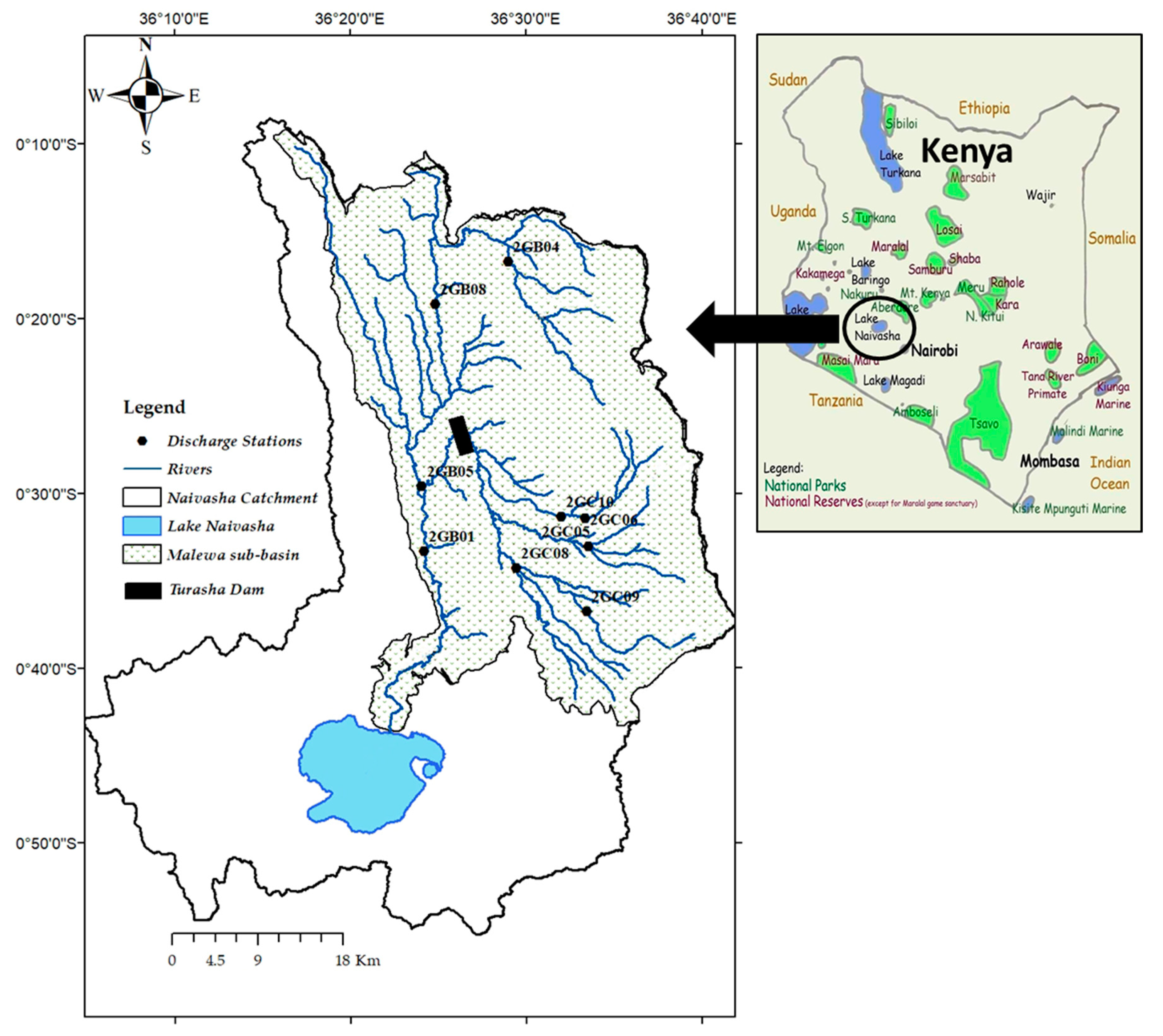
Lake Naivasha catchment is located in the Eastern Rift valley of Kenya at 00°10′ to 00°55′ Latitude South and 36°10′ to 36°40′ Longitude East in zone 37 of the Universal Transverse Mercator (UTM) coordinate system (Figure 1). The lake forms a closed basin without identifiable outlet [21]. The eastern side of the catchment (Aberdare Ranges) has the highest elevation at 3990 m above sea level, while the lowest elevation is about 1980 m [5]. The catchment climate is semi-arid with mean monthly temperatures of around 16 °C and maximum and minimum mean temperatures of 26 °C and 7 °C, occurring in January and August, respectively. Rains occur from March to June (the long season) and short rains are experienced from October to early December. The average yearly rainfall in the lake area is about 600 mm with the high-altitude areas receiving about 1200 to 1500 mm [5]. The rainy seasons are preceded by dry months that span from December to February and from July to September. However, these periods are not constant and may change over the years.
The major rivers in the Lake Naivasha catchment are the Malewa, Gilgil and Karati rivers. The Malewa River is the dominant river responsible for up to 80% of the total inflow into the lake [22] and forms a sub-basin of approximately 1600 km2 in the Naivasha catchment. The study focuses on this sub-basin (Figure 1). There is also a small diversion dam near the Turasha stream outflow to the main Malewa River. This diversion draws and transfers about 1800 m3/day of water to the Lake Nakuru basin (and city) outside the study area. A large portion of the sub-basin land is used for agriculture (both irrigated and rain-fed). Natural vegetation (shrubs, grasses and forests) also cover a large area of the catchment. The main agricultural activities in the basin consist of small-scale crop growing of, for example, pyrethrum, wheat, maize, onions and potatoes. A considerable portion of the study area has been put under pasture and livestock rearing, which is practiced both intensively and extensively.
2.2. Data Procurement
A digital elevation model (DEM) forms the essential input for the provision of topographic information in the basin. An Advanced Space borne Thermal Emission and Reflection Radiometer (ASTER) satellite sensor-based DEM with a resolution of 20 m and WGS_1984 datum for the Lake Naivasha catchment was used. Land use–land cover (LULC) is a major input component of the SWAT model (Version 2012, Texas A&M University, Texas, TX, USA) as it is used in analysis of hydrological response units (HRUs). The characteristics of the various vegetation and land cover types dictate the hydrological response in the area. Based on land cover and land use, SWAT is thus able to compute the canopy storage and the runoff by which soil is eroded into the streams [23]. Therefore, a LULC map with 30-m resolution that was derived from Landsat 7 Enhanced Thematic Mapper (ETM) for the study area [24] was used. The map has 12 general classes and closer visual inspection proved that there was a fair match between the map and the ground LULC. The soil map adopted for use in SWAT was derived from Kenya Soil Survey maps and data. The parameters that were missing in the soil map were identified by field measurement and/or laboratory determination. The hydraulic conductivity, bulk density and the percentages of sand, silt, clay and rock in the soil were derived from soil samples identified during the field expeditions and further determined in the laboratory. Daily precipitation data from 11 rainfall stations plus the minimum and maximum daily temperature data from three stations within or close to the catchment were acquired. It is noticeable that the catchment has a tropical climate with relatively small spatial temperature variations in which there occur no very low (e.g., freezing temperatures) as well as no extremely high temperature (due to the moderate highland altitude 1800–2500 m on the equator). Therefore it is assumed that the temperature data could represent the studied area properly. Additionally, the long term meteorological data such as average solar radiation, relative humidity and wind speed were also provided for the model’s weather data definition. It is notable that relative humidity and wind speed datasets are not needed to provide for the model when the Hargreaves method is selected for determining the potential evapotranspiration.
The River Malewa Basin has several gauge stations (Figure 1) installed for the daily measurement of discharge. These are monitored and managed by the Water Resources Management Authority (WRMA) in Naivasha. Not all gauge stations were in operation, but the ones that had enough data to be used in the modeling were the 2GB04, 2GB05, 2GB08, 2GC04 and 2GC05 stations. The daily discharge data for the years 2004–2017 was obtained from the database of the WRMA. There were no pesticide application data available regarding organochlorine pesticides (OCPs) in the studied area covering this study period. These kinds of pesticides have been banned from import and use in Kenya for many years. However, there is still a risk of finding their residues in the catchment [25]. Therefore, a field survey was conducted to gather information on farm operation management such as cultivation practices, cultivated crops, harvesting methods, pesticides applied, as well as times and amounts of application of these pesticides. The 2016–2017 surveys did not reveal any data on OCPs. Then, a field campaign was carried out in June–July 2016 to measure pesticide content using passive sampling technique (silicon rubber sheets) at 2GB04 and 2GB05 stations (Figure 1), located in the main river as Upper Malewa and Down Malewa [26]. Passive sampling method allows the measurement of low concentrations by collecting the pollutants over a long time period (e.g., some months). Therefore, the samplers were deployed at the sampling stations during June–July according to the relevant passive sampling instructions [26]. After the exposure time, the samples were collected from the sampling stations and after the initial preparations in the lab, the organochlorines residues were analyzed using a gas chromatograph in combination with an electron capture detector (GC-µECD) [26].
Based on the results of these measurements, the residues of methoxychlor, lindane, and endosulfan (sulfate) were found in the Malewa River Basin. It is noticeable that endosulfan-sulfate is the oxidation product of endosulfan as the parent insecticide that was evaluated. However, the possible time and amount of application and physiochemical properties of these pesticides’ parameters, such as soil adsorption coefficient (SKOC), wash-off fraction (WOF), half-life in soil and foliage (HLIFE_S and HLIFE_F) as well as solubility in water (WSOL), were acquired as input to SWAT. Additionally, daily suspended sediment monitoring data were also obtained by installing a Digital Turbidity Sensor (DTS-12, Forest Technology Systems, Victoria, BC, Canada,) in the river at 2GB04 station from April to December 2017. The DTS sensor measurements were taken at 15 min intervals to capture the variations at high temporal resolution. The DTS data were also calibrated against sediment concentration, during suspended sediment sampling campaigns (April–June and September–October, 2017) using a US DH-48 hand-held depth-integrating sampler (US. Geology Survey, Reston, VA, USA).
2.3. Model Setup
The ArcSWAT interface (Version 2012, Texas A&M University, Texas, TX, USA) was used for modeling discharge, sediment and pesticide transport in Malewa River Basin. The model delineates the watershed into sub-basins and Hydrological response units (HRUs). The HRU is defined as a unit of uniform hydrological response and land properties in terms of land cover and use, soil and topography. A sub-basin is defined as an area that is composed of several hydrological response units [27]. Based on the combination of the data fed into the model (e.g., topography, land cover and use, soil properties and weather data), the model uses the HRUs and the sub-basins during its simulation to predict the discharge inflows and outflows as well as the sediment and chemical transport from every sub-basin.
After overlaying the land use, soil and slope maps, 147 HRUs with 22 sub-basins were created. The HRU thresholds were set to 10%, 5% and 10% for land use, soil and slope respectively [7]. The weather data in the model consist of precipitation, temperature, relative humidity, solar radiation and wind speed. These input tables can be either introduced to the model or simulated using a weather generator option in the model. However, as rain data are governing input data that directly influence the results [12], it is important to provide the model with the measured rain data. The model calculates the hydrological parameters for the HRUs, which are linked to the sub-basin’s level and finally routed to the outlet points of the basin [12]. Calibration and validation of the model for discharge data was, respectively, performed from 2007 to 2012 (with a three-year warm-up period from 2004 to 2006) and 2013 to 2017. As sediment and pesticides data time series was short, the model was (only) validated with discharge measurements. The daily sediment data were collected during nine months (April–December, 2017) and pesticides were collected during two months (June–July, 2016) of taking measurements.
Discharge is a key factor in sediment transport, and calibration of the sediment was done on the discharge-calibrated and validated model. The model was calibrated for both daily and monthly data to determine which approach would provide a better output. The Soil Conservation Service (SCS) was used to estimate the surface runoff [6], which is governed by curve number (CN) values. This method is a function of soil infiltration, land use and soil moisture [12] with a larger CN representing higher potential runoff yield, and vice versa. The hydrological process is based on the water balance, which is a function of precipitation, evapotranspiration, quick runoff, irrigation, infiltration rates and lateral flow [27]. The hydrological component of the model at each HRU simulates the hydrological balance using following equation:
where SWt is final soil moisture content (mm), is initial water content (mm), t is time in days, is precipitation (mm), is surface runoff (mm), is Evapotranspiration (mm), is amount of water seeping into the soil profile (mm) and is amount of return flow (mm).
As pesticides move through runoff and sediment, either dissolved in water or attached to soil and sediment particles, monthly and daily sediment calibration was also performed with this calibrated model being used to simulate pesticide movement. The Modified Universal Soil Loss Equation (MUSLE) is applied in the SWAT model for the calculation of sediment yield. This equation is a function of surface runoff and is defined as:
where is the sediment yield (metric tons) of a HRU, is the volume of surface runoff (mm/104·m2), is peak runoff rate (m3/s), is area of the HRU (104·m2), is Universal Soil Loss Equation (USLE) soil erodibility factor, is USLE cover and management factor, is USLE support practice factor, is USLE topographic factor and is coarse fragment factor.
Surface runoff transports adsorbed pesticides in sediment and into the main channels. The adsorbed pesticide loads can be calculated by the following equation:
where is Sediment with adsorbed pesticide in the main channel (kg pesticide/104·m2), is Concentration of sediment on the top soil layer in ton soil, is daily sediment yield (metric tonnes), is the area of the HRU (104·m2), is enrichment ratio of the sediment. The total amount of pesticides is calculated by summing up the adsorbed and the dissolved amounts.
2.4. Model Sensitivity Analysis, Calibration and Validation
Usually, initial modeling with SWAT using default parameters does not produce promising outputs in relation to model inputs [12]. This calls for the model to be calibrated, which involves adjustment of parameters until the simulation results match with the observed data for a specific time period. The identification of the best adjusted parameters for better simulation is achieved with a sensitivity analysis, with the aim to minimize the amount of time consumed trying to calibrate the model. Based on different studies [6,12,15,28], there were various parameters related to discharge, sediment and pesticides transport to be calibrated. The surface runoff lag coefficient (SURLAG) was responsible for the control of the fraction of the total amount of water that entered the outlet in a day (Table 1). The groundwater delay time that controls the amount of time it takes for water to move from the vadose region to the deeper shallow aquifer was affected by the groundwater delay (GW_DELAY) parameter, while the base flow alpha factor (ALPHA_BF) factor governed the discharge recession curve intended to correctly depict the base flow drainage tendencies of the watershed. The parameters related to the channels, such as Manning’s value (CH_N2) and hydraulic conductivity (CH_K2) were also used to adjust the discharge. The flow of water through the soil was regulated by the hydraulic coefficient parameter (SOL_K) and threshold depth outflow from shallow aquifer (GWQMN) was needed for return flow to occur. The model parameters that were used for calibrations and the applied metrics for model performance are presented in Table 1, Table 2, Table 3 and Table 4.
The calibration and uncertainty procedures (SWAT-CUP) tool was used to find the most sensitive parameters in the modeling. In this model, the SUFI-2 algorithm was selected to describe the uncertainty of the parameters based on a uniform distribution assumption. This algorithm is able to perform the approximation at a 95 percent prediction uncertainty level called 95PPU [6]. SUFI-2 initially assumes large uncertainty in the parameters covering all the observed data at 95PPU level. This uncertainty is reduced in subsequent rounds until the difference between the upper and the lower parts of 95PPU—97.5% and 2.5% levels—is minimized and 95PPU includes 80–100% of the observations [10]. The SUFI-2 algorithm uses a Latin hypercube [29] sampling approach where n parameters are combined in a satisfying simulation number (500–1000 runs), with the simulations thereafter being assessed using an objective function [10]. There are several objective functions in SWAT-CUP dealing with model calibration [30]. In this study, the Nash–Sutcliffe coefficient, R squared and percent bias (PBIAS) (Equations (4)–(6)) were used as model performance measures for the assessment of discharge and sediment simulations [31] that permit an appropriate parameter and model performance evaluation.
where is the ith value of observed data, is the ith value of simulated data, is mean value of the observed data and is mean value of the simulated data. The NSE ranges from −∞ to 1. Values for the NSE from 0 to 1 indicate a tolerable level of performance, while values below zero are not acceptable. PBIAS represents the average affinity of the simulated values to be more or less than measured data [31]. The model was calibrated based on the most sensitive parameters (Table 1) for surface discharge data from the sampling stations that had a complete dataset for the period 2004–2012. The model was then validated against the measured data for the period 2013–2017 without further adjustment of the parameters. The results were evaluated for correctness using the suitable model performance statistical measures of PBIAS, NSE and R squared. The model was also calibrated for the sediment simulation by keeping the discharge related parameters fixed and adjusting the sediment related parameters (Table 3) [32]. Finally, as there was a pesticide data shortage, the average monthly data over two months were used to gain insight in the pesticide simulation based on operational management in the basin. Without changing other parameters in the model, the parameters governing pesticide movement were adjusted manually to achieve the best possible match between the model results and the measured pesticides at 2GB04 and 2GB05 station (e.g., Upper and Down Malewa, respectively). The possible times of pesticide applications and cultivation practices were assumed to be in the rainy seasons, when agricultural activities occur. It should be noted that per simulation, only one pesticide can be traced [33], therefore, the model calibration for pesticides was separately performed for methoxychlor, lindane and endosulfan (Table 4).
3. Results
3.1. Discharge Simulation
The sensitivity analysis of the model using SWAT-CUP indicated 16 sensitive parameters related to discharge (Table 1) that could be adjusted to calibrate the model. The results showed that the discharge peaks during the simulations were most sensitive to curve number (CN2) values and the SOL_K parameter, which both vary spatially in the basin, and other parameters were in lower level of sensitivity.
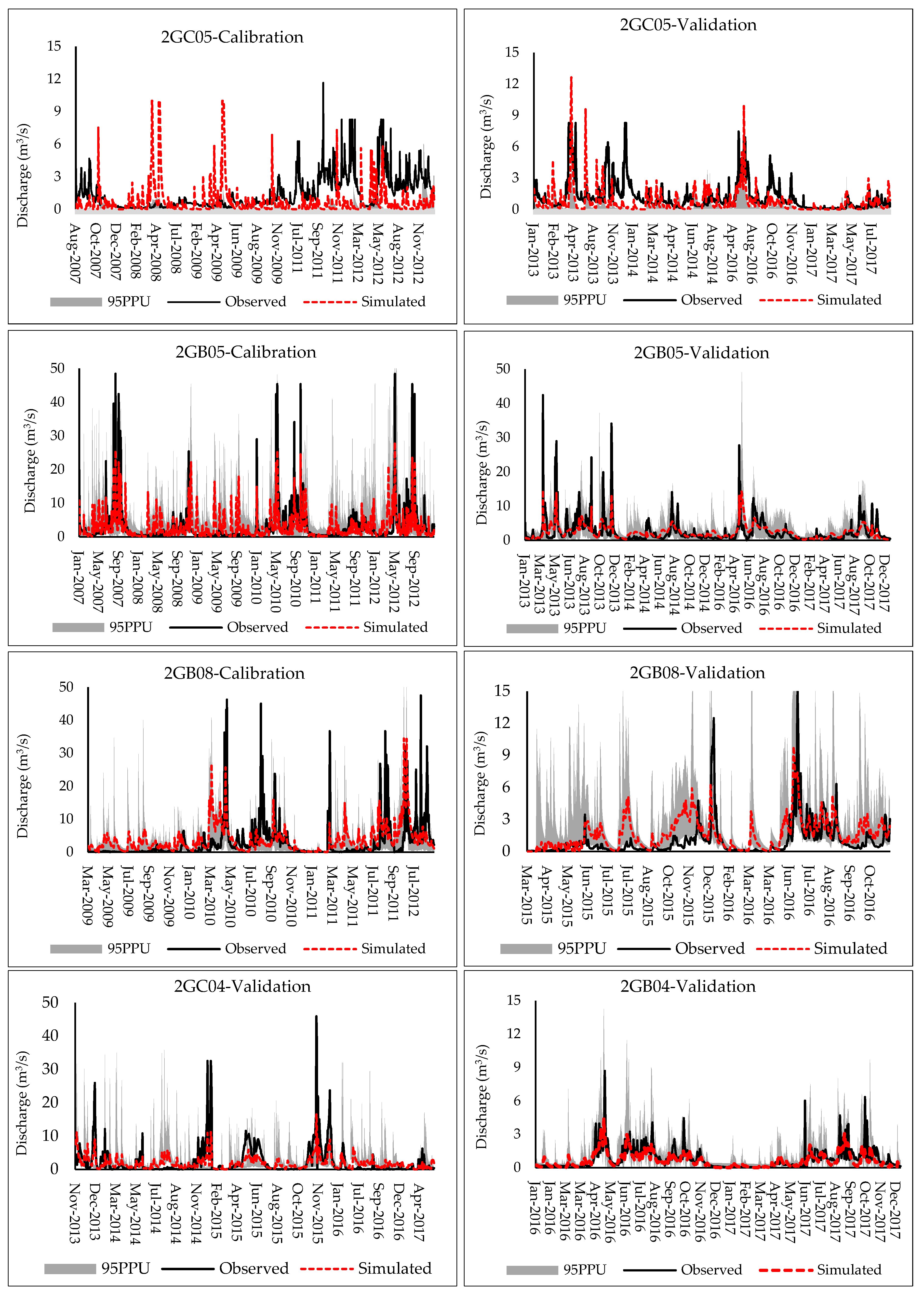
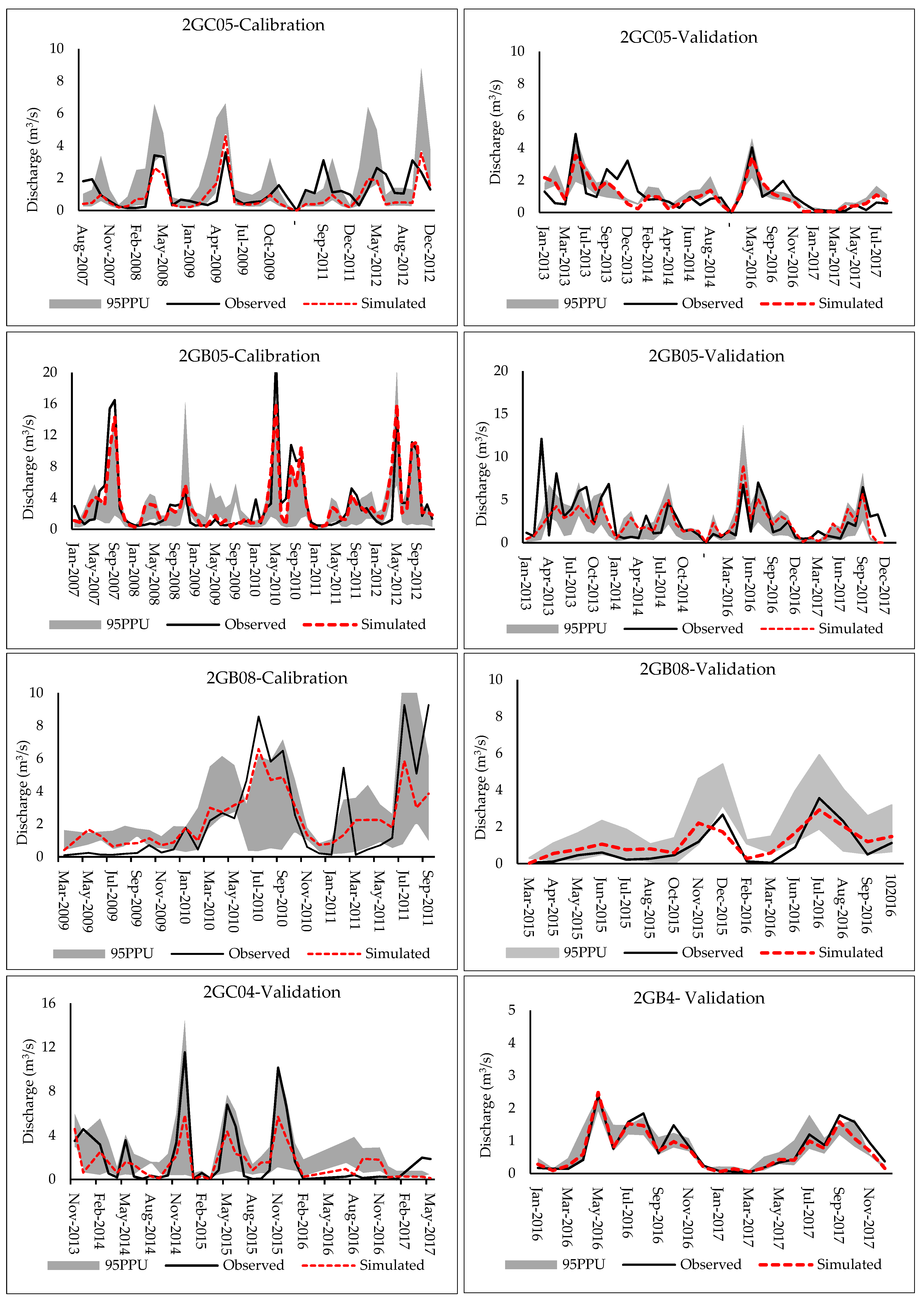
The results of the statistical evaluation of discharge simulations is presented in Table 2. The results of calibration for daily simulation in the gauge stations showed an R2 between 0.61 and 0.05, NSE between −1.20 and 0.47 and up to 50% that based on Moriasi et al. [31] were unsatisfactory. While the monthly simulations with an R2 of 0.70 to 0.86, NSE of 0.51 to 0.64 and within 15% showed satisfactory to very good outputs [31] (Figure 2 and Figure 3). As in some of the stations the time period for daily and monthly calibration was not the same, the PBIAS values were different for daily and monthly simulations. During the validation period also, the results of the daily discharge simulation at the stations varied between 0.28 and 0.60 for R2, between 0.02 and 0.47 for NSE and up to 66% for . Comparing the simulated and measured data for the monthly validation period also showed satisfactory to good results [31]. Generally, the results showed that the output of the model was appropriate. Moreover, the results of the uncertainty analysis showed more than 70 percent of the discharge variations to be bracketed by the 95PPU during both calibration and validation of the monthly simulation, confirming a promising model output [6,30]. Abbaspour et al. [34] introduced a P-factor and an R-factor to quantify the match between simulated and measured data. The percentage of the enclosed observed data is represented by the P-factor while the R-factor shows the thickness of the 95PPU. They also suggested that a P-factor of more than 70 percent and an R-factor of about 1 denote a good result. The results of the monthly simulation revealed a P-factor of more than 80% and an R-factor of 1.1, confirming a satisfying monthly discharge simulation.
3.2. Suspended Sediment Tranpsort Simulation
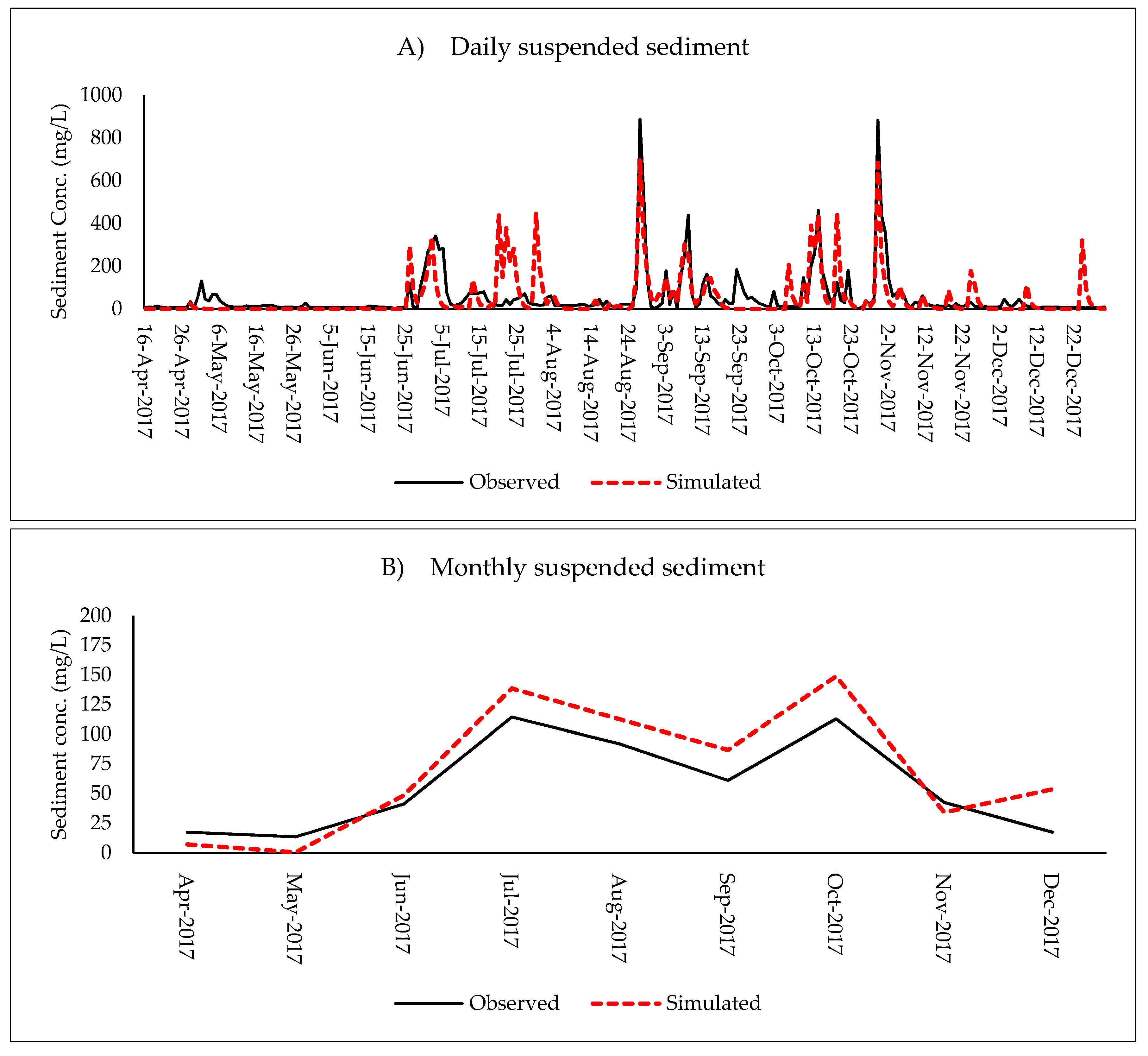
The parameters that were specifically related to sediment loadings from the HRUs and sub-basins that were most sensitive in the model calibration are found as Table 3. The results of sensitivity analysis showed that among these parameters, the most sensitive one was the USLE soil erodibility factor (USLE-K). The soil conservation support practice factor in the USLE equation (USLE_P) was in the second rank and depends on land use—land cover of the area. This parameter represents the human interventions with the soil, and the crop management processes that take place in the basin. The parameters of channel cover (CH_COV) and channel erodibility (CH_EROD) also showed high sensitivity and could influence the amount of simulated sediment production due to sediment loss from the channels [12]. The comparison of daily and monthly results showed that simulated and measured sediment matched well (Figure 4), with the monthly simulation exhibiting better results than the daily steps. The statistical results of model performance also showed the R2 = 0.51, NSE = 0.44 and |PBIAS| = 19% for the daily and R2 = 0.60, NSE = 0.70 and |PBIAS| = 19% for the monthly simulations that both are in range of satisfactory to good [6,31].
3.3. Pesticides Transport Simulation
Although data on organochlorine pesticides loading in the rivers of the Lake Naivasha catchment were limited for a full model calibration and validation [25], the attempt at simulating the fate of the pesticide residues of methoxychlor, lindane and endosulfan using in-situ measured concentrations could help gain insight into pesticide application and mobility in the study area. The sensitive parameters in the model calibration of pesticide residues are presented in Table 4. The results of this calibration demonstrate that application efficiency (AP_EF) forms the most sensitive parameter when simulating the pesticides. HLIFE_S and HLIFE_F that show half-life duration (days) of the pesticides in the soil and on the foliage, respectively, also proved highly sensitive in the calibration.
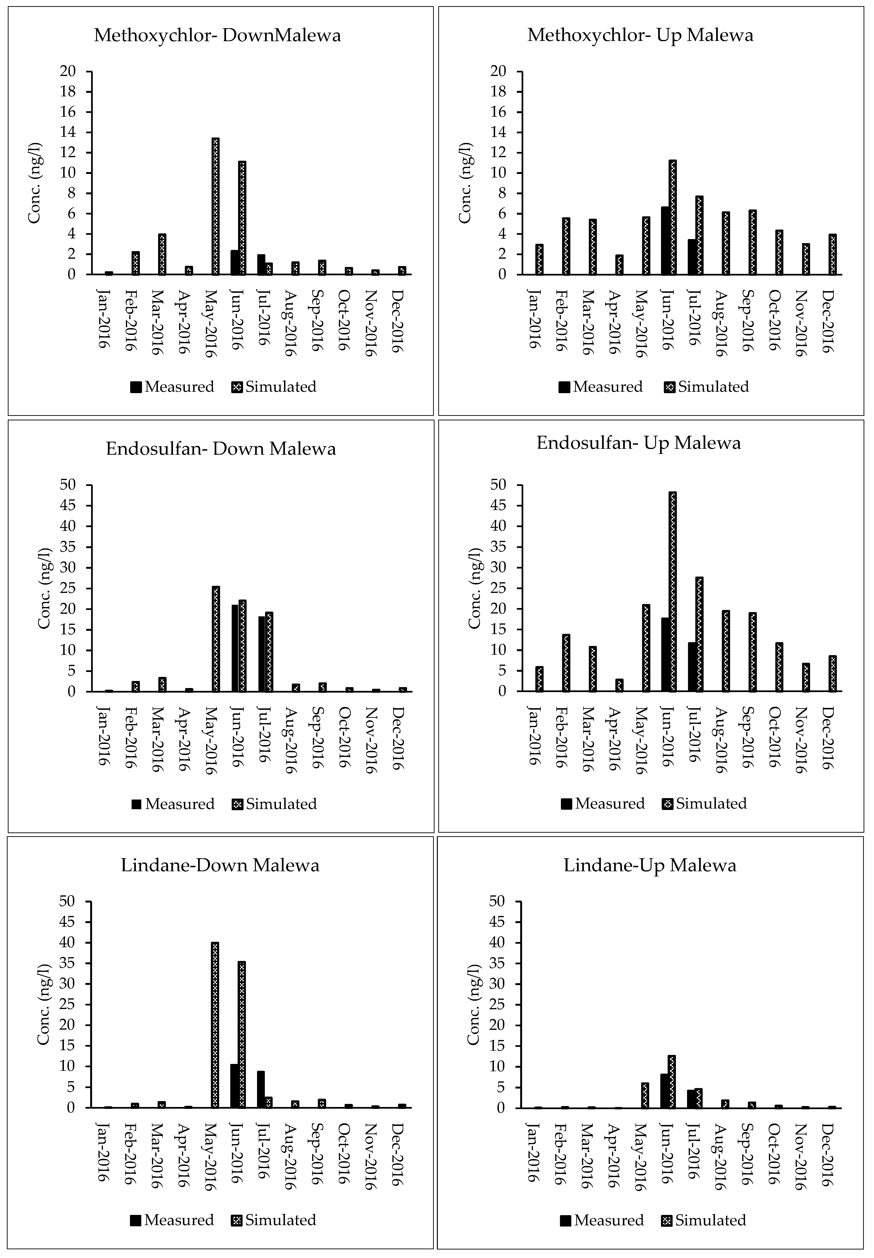
Correlation between the simulated and measured pesticide residue concentrations at the Upper Malewa and Down Malewa sites is represented in Table 2 and Figure 5. The results of pesticide transport modeling are based on data converted from mass-transported amounts to pesticide concentrations. It was found that most applications and consequently the highest concentrations of the studied pesticide residues occurred from May to mid-July during the simulation period. The simulation results showed the month May to have the highest pesticide loading into the rivers for all studied pesticides. According to the results of simulations that are supported by measured data, endosulfan had the highest concentration on average, i.e., from 22 to 28 ng/L. During June and July, the model mostly overestimated pesticide residue concentrations. However, the model simulated a valid and observed trend in pesticide variation based on the measured data, confirming the capability of the SWAT model to evaluate the rainfall–runoff-based transport of pesticide residues.
4. Discussion
Rainfall–runoff and river discharge are the main driving force behind the movement of sediment and pesticides through the basin. Therefore, an appropriate calibration of the SWAT model, which is a physically based model, can play an important role in final outcomes. By applying SWAT-CUP as a tool for calibrating the model, the values of the observed and the model simulated monthly discharge for the calibration period (2007–2012) were found to display a satisfactory statistical agreement. The daily simulation results were not as good as the monthly ones. In fact, the SWAT model generally displays better results over longer steps than short (e.g., daily or hourly) steps. The studies by Liu et al. [35] and Spruill et al. [36] also demonstrated that the model had a better performance in monthly and yearly simulations than the daily steps that can support the results of this study. This may be attributed to the fact that daily rainfall–runoff processes display higher variability rather than aggregated data on monthly basis in which the average of accumulated data is taken and the local and any short-term variations are smoothed while the general trend is still followed. The studied basin has very diverse land properties (e.g., slope, land cover and use, soil), which may influence the response to rain events in hydrological units on a daily scale. Different sub-basins have varying features and the sensitive parameters for discharge simulation may differ from one to another. However, the results of several studies [12,15,28,37] demonstrate that the SCS curve number for soil moisture condition (CN2.mgt) is the most or, at least, one of the most sensitive parameters in model calibration for discharge simulation, which is supported by the findings of this study. This landscape parameter can affect the peak flow [6] and varies across hydrological units, based on their land use and soil properties, which can affect their potential for runoff from rainfall events. Soil hydraulic conductivity (SOL_K) follows as next most sensitive parameter in discharge simulation, showing the potential for soil infiltration by either transforming the rain into surface discharge or conveying the water down into the soil layers. It should be noted that the Lake Naivasha catchment has diverse soil properties, with high spatial variability in the soil parameters (e.g., SOL_K of between 4 and 41 mm/h). Moreover, although this is a simplified explanation of the relation between surface and groundwater, GW_DELAY, GWQMN, GW_REVAP, and CH_K2 were used to simulate their interaction in the modeling [6,38].
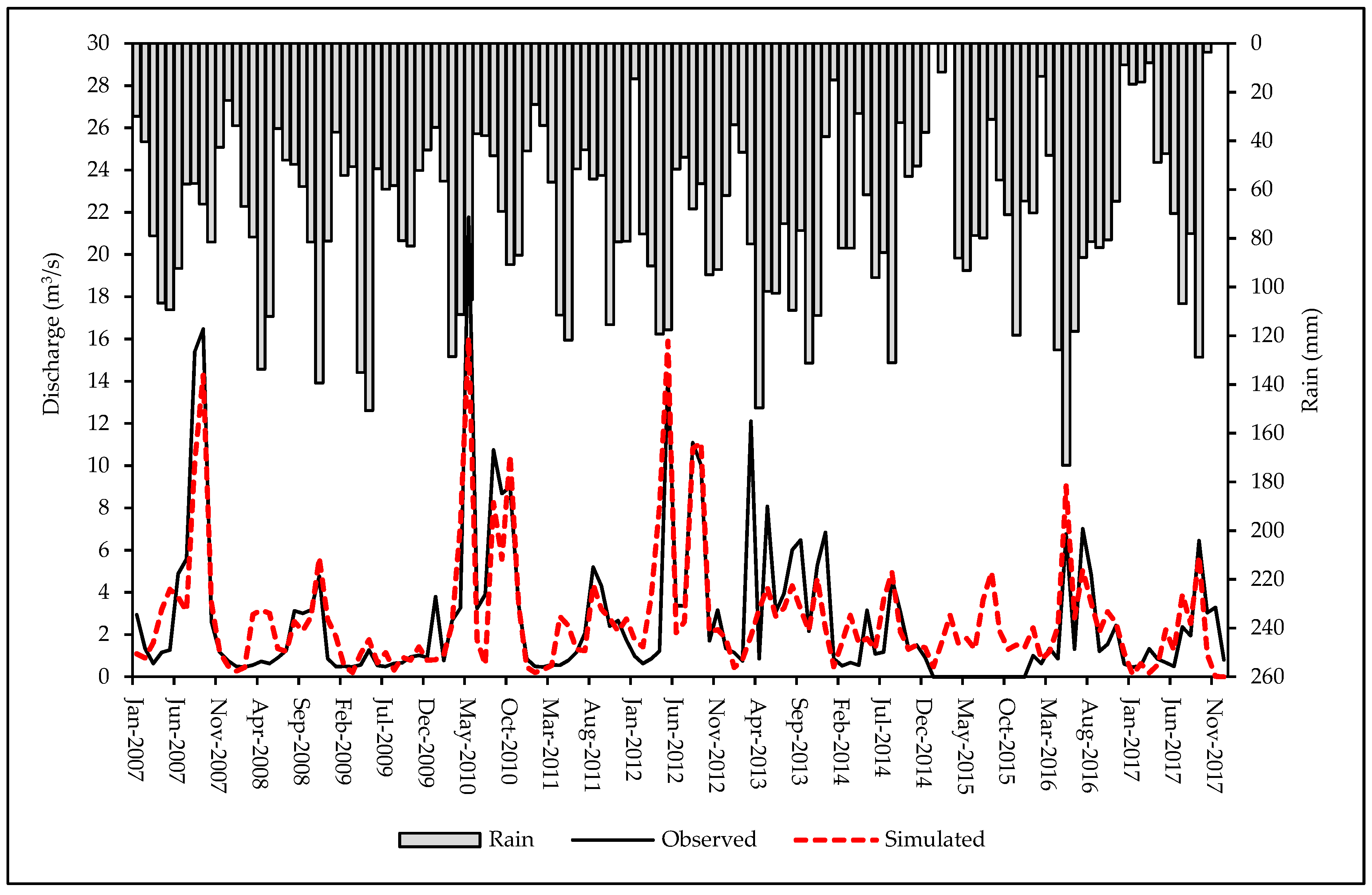
The diagram of the calibration (2007–2012) and validation (2013–2017) periods shown in Figure 6 demonstrates agreement between discharge and precipitation with slight underestimation by the model in the wet seasons and overestimation in the dry seasons. The statistical evaluation measurements of the model’s monthly simulations are also acceptable (R2 > 0.46 and NSE > 0.44), which means that the selected range of model parameters matches the basin condition. The reason that the dry seasons are slightly overestimated by the model may be caused by the curve number method not being able to generate runoff accurately during prolonged dry periods despite independent rainfall events occurring during that time [39].
The simulation of sediment production and transport showed that most of the sediment is produced during events of high rainfall and discharge. The discharge is a proxy for soil erosion. As more soil is eroded the sediment amounts in the stream channels will increase. This is in agreement with findings by Asres and Awulachew [40], who explored sediment yield in the Gumera watershed of Ethiopia. The calibration of the model for sediments over nine months captured both the wet and dry season in the area. Normally, the main rainy period is during April–June, but because of a short drought in the catchment, the rainy season was delayed to July–October. Comparing simulation results against the observed sediment loads confirmed that there was more sediment production in this period, receding from October onwards (Figure 4). Exploring the daily results of the sediment estimation showed that although the R2 of simulation was almost promising (R2 = 0.51), the results were not as good as for the monthly simulations. The conclusion is that the model does not satisfactorily detect discharge and sediments produced by single storms in a day. It is more accurate in predicting sediment yield by a series of continuous rainfall events.
However, statistical comparison between the monthly simulated sediment loads and the observed loads demonstrated that the performance of the model was reasonable. Soil erosion in SWAT is based on the Modified Universal Soil Loss Equation (MUSLE) [41]. Sensitivity analysis and calibration of this equation in the Malewa basin was explored by Odongo et al. [5] and the results showed that the model could reasonably be applied for sediment simulation. Moreover, comparing the daily results of this study with their results based on some events that occurred during September to October showed that the range of sediment yields were comparable. Two of the most sensitive variables that were used in the model calibration for estimation of sediment transport were USLE-K and USLE_P. The first factor shows the inherent susceptibility of soil to erosion by water and can be calculated as the eroded soil mass per unit rainfall erosivity and area [42]. This parameter can be estimated from soil properties such as soil texture, organic matter and structure [42]. USLE_P is related to soil conservation conditions such as land contouring, tillage and terracing and demonstrates the effect of surface management on erosion processes during runoff events. But as it is difficult to determine the real value for this factor, a calibrated or default value is applied, which is not to be recommended [42]. Changing these two factors to a calibration factor in the SWAT model allows matching between measured and simulated data, while these parameters in fact need to be derived from soil or land surface properties. Therefore, as these factors are not single parameters that can be changed by calibration, it is understood that the SWAT model simplifies the estimation of soil erosion and sediment yield.
It should be noted that calibration of the model on a large scale is associated with many uncertainties [43], with the main uncertainty possibly being caused by agricultural management activities, which can influence the sediment loading [6]. Nonetheless, calibrating the model using a high-quality dataset that was recorded automatically and compiled with rainfall events should aid the achieving of a proper sediment estimation. The simulation of the sediment load depends on several factors in the watershed. These factors could be physiographical, the contribution of the watersheds to the stream flow that moves to the outlet, the quantity of the highest rate of runoff, the intensity of precipitation and concentration of the sediment [12]. The SWAT Model produces the sediment results per sub-basin, making analysis at sub-basin level possible. The possible causes leading to various sediment production fluxes in the catchment were investigated to ascertain the different factors other than the precipitation amounts and geographical factors that could influence the sediment production rate in each sub-basin. The SWAT model uses the Thiessen polygon method to allocate the nearest rainfall station to a sub-basin. The variations in rainfall around the basin could lead to different amounts of sediments being produced in the catchment. Moreover, sub-basins with more agricultural activity as well as high slopes could have higher rate of sediment yield than other parts. This finding confirms that agricultural activity on the higher slopes of a sub-basin encourages soil erosion and hence sediment production.
Integrating the results of discharge and sediment simulations for the daily and monthly steps confirmed that the monthly simulations were more reliable than daily simulations which was overall unsatisfactory. By selecting the monthly time step for estimating the pesticide load, it became possible to evaluate pesticide transport. There are several studies that have applied the SWAT model successfully to simulate pesticides transport in catchments [6,11,16,44]. This proves the capability of this model for exploring chemical transport by water. In this study, because of limited data, the model validation of the pesticides was not done which can cause uncertainty of the results. However, as other studies in this catchment about organochlorine pesticides used only grab samples analysis (spot measurements) [25], the modeling in this study can be considered as a pilot application which improves our insights into the pesticides transport in the catchment. Moreover, use of passive sampling that allows measuring low concentrations of pesticide residues, helped the improvement of the data for more reliable modelling and assessment.
From the sensitive parameters in pesticide simulations (Table 4), it can be seen that increasing the application efficiency (AP_EF) caused an increase in the quantity of pesticide that entered the system, consequently increasing the pesticide load as well. Comparing the effect that this parameter had on the pesticides simulation with the study by Chen et al. [6] supported this finding. The pesticide percolation coefficient (PERCOP) was also seen as an important parameter to be defined and has been reported in different studies [11], however 0.50 was found to be the best match with the simulation. The next parameter that had most effect on the results was HLIFE_S, which controls the pesticides degradation process. Obviously, by increasing this parameter, more pesticide residue has a chance to be washed out and reach the streams during the runoff events [6]. Normally organochlorine pesticides have a long half-life and, depending on the conditions can remain in the environment from some months to some years [45]. Lindane (for instance), also known as gamma-hexachlorocyclohexane (γ-HCH), has various isomers (e.g., α-HCH, β-HCH, γ-HCH, δ-HCH) that are used as insecticide for protecting fruits, vegetables and animals. These isomers are very stable in environment (half-life of years) and are categorized as the persistent organic pollutants (POPs) by the Stockholm Convention on persistent organic pollutants [46]. The environmental fate and distribution of lindane, like that of other organic chemicals, is related to environmental conditions and its interactions with other environmental compartments as well as the physical chemical properties of the isomers [47]. Methoxychlor also binds strongly to soil particles and might be transported by wind and rain in eroded polluted soils or can be washed to water bodies by runoff. Depending upon the existence of photosensitizers, methoxychlor can have a half-life of 4.5 months to half-life of less than 5 h [45]. Half-life of methoxychlor in sediments in anaerobic is more than 28 days and aerobic is more than 100 days [45]. Endosulfan has some isomers such as α-endosulfan, β-endosulfan and endosulfan sulfate that have high acute toxicity and could remain in environment. The main metabolite of endosulfan degradation in soil is endosulfan sulfate that is the oxidation product of endosulfan [48]. The fate of endosulfan is strongly governed by environmental conditions. When it is released to air, the vapor-phase endosulfan can be degraded in the atmosphere with half-life of about 2 days [49]. When released to soil, based on its SKOC values, it can have an average to only low mobility and is not expected to volatize from the soil. In this condition, half-lives of 32 and 150 days for aerobic and anaerobic soils have been reported [49]. If released to water, the suspended solids could adsorb the endosulfan and under aerobic and anaerobic conditions the half-life varies between 2 and 8 days, respectively [49]. Therefore, with regard to these various physico chemical features and behaviors of the studied pesticides, the difference in observed and simulated results can be understood.
Moreover, organochlorine pesticides also have a low tendency for solubility in water, making this feature to be found in small values of WSOL parameter. The sensitivity of SKOC differed among the pesticides depending on the kind of pesticide. By increasing this parameter, its sensitivity was decreased. Therefore, lindane was more sensitive to changing SKOC than methoxychlor and endosulfan. It is noticeable when SKOC is increased in a specific kind of pesticide, the expected amount of washed pesticide will decrease [44]. This issue can also affect the WOF parameter. Therefore, selecting a proper amount of SKOC can influence the coherence between simulated and measured pesticide values.
Generally, there was a better match between estimated and measured concentrations in the Upper Malewa (2GB04) than in the Down Malewa (2BG05) station. One of the reasons that may explain this result is that at the upper site it takes less time for runoff and pesticides to reach the outlet of the subbasin and consequently there is a quicker response to changes. In moving from Upper Malewa to Down Malewa, the hydrological contribution increases, as does the complexity of accurately predicting the concentrations of pesticides. This issue is added to the increasing time for an amount of the pesticides to reach the basin outlet, affecting the mechanism of pesticide conveyance and the breakdown of pesticides into soluble and sorbed phases [44]. This may also be true for the application time. Changing the time of application of pesticides impacts on the arrival of the pesticides at the basin outlet [11] and consequently changes the amount of pesticide that leaches from the soil surface particles. Therefore the best time to achieve good results in this study was the 15th of May, which coincided with the rainy season and the time of agricultural activity and pesticide application. It should be noted that defining a fixed application operation in such a vast basin is practically impossible [11,50]. The timing may vary depending on the farmers willingness, weather conditions, plant properties and existing pests that may change spatially and temporally [6]. This will influence the fluctuation in pesticides in the streams and, accordingly, the uncertainties of the simulations.
Additionally, the accuracy of pesticide simulations strongly depends on the hydrology calibration of the model [14]. In fact, because of the challenges that are associated with the large numbers of input data, their variability and consequently the uncertainties that arise, satisfactory modeling is always wrought with difficulties [51]. Simulating pesticides in this study after hydrological calibration and validation showed that the main pesticide loadings occurred at the time of peaks in runoff and sediment loads. The main governing factor in runoff and sediment producing is the major rainfall occurring during May–June–July. Of the pesticides studied, lindane is least likely to adhere to soil and sediment particles. This leads to the conclusion that lindane will be mostly translocated by runoff. In contrast, methoxychlor and endosulfan have a large SKOC, meaning that they have a high tendency to cling to be absorbed by soil and sediment particles and consequently the main force of transport will be via erosion and sediment loading. This means that the better hydrological processes are modelled, the more reliable the pesticide results could be.
5. Conclusions
In this study, a modeling approach using SWAT was conducted to simulate the discharge, sediment loading and pesticides residues transport regarding lindane, methoxychlor and endosulfan in the Malewa River Basin. The SWAT-CUP tool was used to calibrate the model for discharge and suspended sediment simulations. It was found that 15 parameters affected calibration, of which the CN parameter proved most sensitive to spatial changes. The statistical analysis showed that both the calibration and validation periods of discharge were promising. Moreover, calibration of the model for monthly sediment simulation showed that, despite slightly overestimating the results of the simulation, the overall performance of the model could be rated acceptable. The average monthly sediment production and the differences in sediment amounts in the sub-basins could be explained by precipitation, slope variation and land use properties in the basin. Moreover, the use of a digital turbidity sensor (DTS-12) is recommended for calibration of the sediment yield sub-model in SWAT. Finally, simulating pesticides could provide a good insight into historical pesticide application in the basin. Some of the parameters, namely SKOC, WOF, HLIFE_F, HLIFE_S, WSOL and AP_EF, were sensitive to calibration of the pesticide sub-model. Of these, AP_EF showed the highest sensitivity towards all the pesticides. The results reveal that the amounts of pesticide generally increased from the Upper Malewa to the Down Malewa. Passive sampling was judged to be an essential method in detecting low concentrations of pesticide residues in runoff of the Malewa River. In this study, we used a limited—but considered high quality (passive sampling with low detection limit)—data set of pesticide measurements in the basin. Further investigation of the fate and transport of pesticides using longer series of data and use of more advanced physicochemical models is recommended to overcome the uncertainty that arises from limited in-situ measurements combined with simplifying model formulations.
Author Contributions
Y.A. designed and conducted the fieldwork and data collection, model calibration-validation and writing the paper. C.M.M. and Y.A. developed the research objectives and conducting of methods. C.M.M. also verified the model simulation results and contributed to editing of the paper. W.M. was involved in the field data collection and the model simulations.
Funding
This research received no external funding.
Acknowledgments
The authors thank the Water Resources Management Authority (WRMA) and WWF in Naivasha that provided the discharge data and contributed in the passive sampling campaign. The Laurel flower farm (Naivasha) for helping us with instruments maintenance.
Conflicts of Interest
The authors declare no conflict of interest.
References
- Harper, D.M.; Morrison, E.H.J.; Macharia, M.M.; Mavuti, K.M.; Upton, C. Lake naivasha, kenya: Ecology, society and future. Freshw. Rev. 2011, 4, 89–114. [Google Scholar] [CrossRef]
- Warren, N.; Allan, I.J.; Carter, J.E.; House, W.A.; Parker, A. Pesticides and other micro-organic contaminants in freshwater sedimentary environments—A review. Appl. Geochem. 2003, 18, 159–194. [Google Scholar] [CrossRef]
- Vigiak, O.; Malago, A.; Bouraoui, F.; Vanmaercke, M.; Obreja, F.; Poesen, J.; Habersack, H.; Feher, J.; Groselj, S. Modelling sediment fluxes in the danube river basin with SWAT. Sci. Total Environ. 2017, 599–600, 992–1012. [Google Scholar] [CrossRef]
- Panuwet, P.; Siriwong, W.; Prapamontol, T.; Ryan, P.B.; Fiedler, N.; Robson, M.G.; Barr, D.B. Agricultural pesticide management in thailand: Situation and population health risk. Environ. Sci. Policy 2012, 17, 72–81. [Google Scholar] [CrossRef] [PubMed]
- Odongo, V.O.; Onyando, J.O.; Mutua, B.M.; van Oel, P.R.; Becht, R. Sensitivity analysis and calibration of the modified universal soil loss equation (musle) for the upper malewa catchment, kenya. Int. J. Sediment Res. 2013, 28, 368–383. [Google Scholar] [CrossRef]
- Chen, H.; Luo, Y.; Potter, C.; Moran, P.J.; Grieneisen, M.L.; Zhang, M. Modeling pesticide diuron loading from the san joaquin watershed into the sacramento-san joaquin delta using SWAT. Water Res. 2017, 121, 374–385. [Google Scholar] [CrossRef] [PubMed]
- Ben Salah, N.C.; Abida, H. Runoff and sediment yield modeling using SWAT model: Case of wadi hatab basin, central tunisia. Arab. J. Geosci. 2016, 9, 579. [Google Scholar] [CrossRef]
- Borah, D.K.; Bera, M. Watershed-scale hydrologic and nonpoint-source pollution models: Review of applications. Am. Soc. Agric. Eng. 2004, 47, 789–803. [Google Scholar] [CrossRef]
- Scopel, C. SWAT: Soil & Water Assessment Tool. ArcGIS Blog. Available online: https://www.esri.com/arcgis-blog/products/product/water/swat-soil-water-assessment-tool/ (accessed on 15 February 2018).
- Abbaspour, K.C.; Yang, J.; Maximov, I.; Siber, R.; Bogner, K.; Mieleitner, J.; Zobrist, J.; Srinivasan, R. Modelling hydrology and water quality in the pre-alpine/alpine thur watershed using SWAT. J. Hydrol. 2007, 333, 413–430. [Google Scholar] [CrossRef]
- Bannwarth, M.A.; Sangchan, W.; Hugenschmidt, C.; Lamers, M.; Ingwersen, J.; Ziegler, A.D.; Streck, T. Pesticide transport simulation in a tropical catchment by SWAT. Environ. Pollut. 2014, 191, 70–79. [Google Scholar] [CrossRef]
- Dutta, S.; Sen, D. Application of SWAT model for predicting soil erosion and sediment yield. Sustain. Water Res. Manag. 2017, 4, 447–468. [Google Scholar] [CrossRef]
- Ligaray, M.; Kim, M.; Baek, S.; Ra, J.-S.; Chun, J.; Park, Y.; Boithias, L.; Ribolzi, O.; Chon, K.; Cho, K. Modeling the fate and transport of malathion in the Pagsanjan-Lumban basin, Philippines. Water 2017, 9, 451. [Google Scholar] [CrossRef]
- Luo, Y.; Zhang, X.; Liu, X.; Ficklin, D.; Zhang, M. Dynamic modeling of organophosphate pesticide load in surface water in the northern San Joaquin Valley watershed of California. Environ. Pollut. 2008, 156, 1171–1181. [Google Scholar] [CrossRef] [PubMed]
- Mahzari, S.; Kiani, F.; Azimi, M.; Khormali, F. Using SWAT model to determine runoff, sediment yield and nitrate loss in gorganrood watershed, Iran. Ecopersia 2016, 4, 1359–1377. [Google Scholar] [CrossRef]
- Folle, S.M. SWAT Modeling of Sediment, Nutrients and Pesticides in the Le-Sueur River Watershed, South-Central Minnesota. Ph.D. Dissertation, Uniersity of Minesota, Minneapolis, MN, USA, 2010. [Google Scholar]
- Parker, R.; Arnold, J.G.; Barrett, M.; Burns, L.; Carrubba, L.; Neitsch, S.L.; Snyder, N.J.; Srinivasan, R. Evaluation of three watershed-scale pesticide environmental transportat and fate models. J. Am. Water Res. Assoc. 2007, 43, 1424–1443. [Google Scholar] [CrossRef]
- Winchell, M.F.; Peranginangin, N.; Srinivasan, R.; Chen, W. Soil and water assessment tool model predictions of annual maximum pesticide concentrations in high vulnerability watersheds. Integr. Environ. Assess. Manag. 2018, 14, 358–368. [Google Scholar] [CrossRef] [PubMed]
- Arnold, J.G.; Moriasi, D.N.; Gassman, P.W.; Abbaspour, K.C.; White, P.S.; Srinivasan, R.; Santhi, C.; Harmel, R.D.; van Griensven, A.; Van Liew, M.W.; et al. SWAT: Model use, calibration and validation. Am. Soc. Agric. Biol. Eng. 2012, 55, 1491–1508. [Google Scholar]
- Wang, W.; Neuman, S.P.; Yao, T.; Wierenga, P.J. Simulation of large-scale field infiltration experiments using a hierarchy of models based on public, generic, and site data. Vadose Zone J. 2003, 2, 297–312. [Google Scholar] [CrossRef]
- Xu, T.Z. Water Quality Assessment and Pesticide Fate Modeling in the Lake Naivasha Area, Kenya. Master’s Thesis, University of Twente, Enschede, The Netherlands, 1999. [Google Scholar]
- Becht, R.; Odada, E.; Higgins, S. Lake Naivasha experience and lessons learned brief. Int. Water Learn. Exch. Res. Net 2010, 2, 277–298. [Google Scholar]
- Meins, F.M. Evaluation of Spatial Scale Alternatives for Hydrological Modelling of the Lake Naivasha Basin, Kenya. Master’s Thesis, University of Twente, Enschede, The Netherlands, 2013. [Google Scholar]
- Odongo, V.O.; Mulatu, D.W.; Muthoni, F.K.; van Oel, P.R.; Meins, F.M.; van der Tol, C.; Skidmore, A.K.; Groen, T.A.; Becht, R.; Onyando, J.O.; et al. Coupling socio-economic factors and eco-hydrological processes using a cascade-modeling approach. J. Hydrol. 2014, 518, 49–59. [Google Scholar] [CrossRef]
- Gitahi, S.M.; Harper, D.M.; Muchiri, S.M.; Tole, M.P.; Ng’ang’a, R.N. Organochlorine and organophosphorus pesticide concentrations in water, sediment, and selected organisms in Lake Naivasha (Kenya). Hydrobiologia 2002, 488, 123–128. [Google Scholar] [CrossRef]
- Abbasi, Y.; Mannaerts, C.M. Evaluating organochlorine pesticide residues in the aquatic environment of the lake naivasha river basin using passive sampling techniques. Environ. Monit. Assess. 2018, 190, 349. [Google Scholar] [CrossRef]
- Neitsch, S.L.; Arnold, J.G.; Kiniry, J.R.; Williams, J.R. Soil & Water Assessment Tool, Theoretical Documentation; Technical Report No. 406; Texas A&M University: Texas, TX, USA, 2011. [Google Scholar]
- Zettam, A.; Taleb, A.; Sauvage, S.; Boithias, L.; Belaidi, N.; Sánchez-Pérez, J. Modelling hydrology and sediment transport in a semi-arid and anthropized catchment using the SWAT model: The case of the Tafna river (northwest Algeria). Water 2017, 9, 216. [Google Scholar] [CrossRef]
- MCkay, M.D.; Beckma, R.J.; Conover, W.J. A comparision of three methods for selelcting valuses of input variables in the analysis of output from a computer code. Am. Stat. Assoc. Am. Soc. Qual. 2000, 42, 55–61. [Google Scholar]
- Abbaspour, K.C. SWAT-CUP: SWAT Calibration and Uncertainty Programs—A User Manual; Swiss Federal Institute of Aquatic Science and Technology, Eawag: Dübendorf, Switzerland, 2015. [Google Scholar]
- Moriasi, D.N.; Gitau, M.W.; Pai, N.; Daggupati, P. Hydrologic and water quality models: Performance measures and evaluation criteria. Am. Soc. Agric. Biol. Eng. 2015, 58, 1763–1785. [Google Scholar]
- Malone, R.W.; Yagow, G.; Baffaut, C.; Gitau, M.W.; Qi, Z.; Amatya, D.M.; Parajuli, P.B.; Bonta, J.V.; Green, T.R. Parameterization guidelines and considerations for hydrologic models. Am. Soc. Agric. Biol. Eng. 2015, 58, 1681–1703. [Google Scholar]
- Arnold, J.G.; Kiniry, J.R.; Srinivasan, R.; Williams, J.R.; Haney, E.B.; Neitsch, S.L. Soil & Water Assessment Tool Input-Output Documentation; TR-439; Texas Water Resources Institute: Texas, TX, USA, 2013. [Google Scholar]
- Abbaspour, K.C.; Rouholahnejad, E.; Vaghefi, S.; Srinivasan, R.; Yang, H.; Kløve, B. A continental-scale hydrology and water quality model for europe: Calibration and uncertainty of a high-resolution large-scale SWAT model. J. Hydrol. 2004, 524, 733–752. [Google Scholar] [CrossRef]
- Liu, Y.; Yang, W.; Yu, Z.; Lung, I.; Gharabaghi, B. Estimating sediment yield from upland and channel erosion at awatershed scale using SWAT. Water Res. Manag. 2015, 29, 1399–1412. [Google Scholar] [CrossRef]
- Spruill, C.A.; Workman, S.R.; Taraba, J.L. Simulation of daily stream discharge from small watersheds using the SWAT model. Am. Soc. Agric. Biol. Eng. 2000, 1, 1431–1439. [Google Scholar] [CrossRef]
- Dasa, S.K.; Nga, A.W.M.; Perera, B.J.C. Sensitivity analysis of SWAT model in the yarra river catchment. In Proceedings of the 20th International Congress on Modelling and Simulation, Adelaide, Australia, 1–6 December 2013. [Google Scholar]
- Traum, J.A.; Phillips, S.P.; Bennett, G.L.; Zamora, C.; Metzger, L.F. Documentation of a Groundwater Flow Model (SJRRPGW) for the San Joaquin River Restoration Program Study Area, California; Scientific Investigations Report 2014-5148; United States Geological Survey (USGS): Reston, VA, USA, 2014.
- Qiu, L.; Zheng, F.; Yin, R. SWAT-based runoff and sediment simulation in a small watershed, the loessial hilly-gullied region of china: Capabilities and challenges. Int. J. Sediment Res. 2012, 27, 226–234. [Google Scholar] [CrossRef]
- Asres, M.T.; Awulachew, S.B. SWAT based runoff and sediment yield modelling: A case study of the gumera watershed in the blue nile basin. Ecohydrol. Hydrobiol. 2010, 10, 191–199. [Google Scholar] [CrossRef]
- Shen, Z.Y.; Gong, Y.W.; Li, Y.H.; Hong, Q.; Xu, L.; Liu, R.M. A comparison of wepp and SWAT for modeling soil erosion of the Zhangjiachong watershed in the Three Gorges Reservoir area. Agric. Water Manag. 2009, 96, 1435–1442. [Google Scholar] [CrossRef]
- Renschler, C.S.; Mannaerts, C.M.; Diekkruger, B. Evaluating spatial and temporal variability in soil erosion risk—Rainfall erosivity and soil loss ratios in Andalusia, Spain. Catena 1999, 34, 209–225. [Google Scholar] [CrossRef]
- Ficklin, D.L.; Luo, Y.; Zhang, M. Watershed modelling of hydrology and water quality in the Sacramento River watershed, California. Hydrol. Process. 2013, 27, 236–250. [Google Scholar] [CrossRef]
- Kannan, N.; White, S.M.; Worrall, F.; Whelan, M.J. Pesticide modelling for a small catchment using SWAT-2000. J. Environ. Sci. Health B 2006, 41, 1049–1070. [Google Scholar] [CrossRef] [PubMed]
- Agency for Toxic Substances and Disease Registry (ATSDR). Toxicological Profile for Methoxychlor; U.S. Department of Health and Human Services Public Health Service: Atlanta, GA, USA, 2002.
- Stockholm Convention on Persistent Organic Pollutants (pops), Text and Annexes; The Secretariat of the Stockholm Convention on Persistent Organic Pollutants: Geneva, Switzerland, 2009.
- Agency for Toxic Substances and Disease Registry (ATSDR). Toxicological Profile for Hexachlorocyclohexane; U.S. Department of Health and Human Services Public Health Service: Atlanta, GA, USA, 2005.
- Weber, J.; Halsall, C.J.; Muir, D.; Teixeira, C.; Small, J.; Solomon, K.; Hermanson, M.; Hung, H.; Bidleman, T. Endosulfan, a global pesticide: A review of its fate in the environment and occurrence in the arctic. Sci. Total Environ. 2010, 408, 2966–2984. [Google Scholar] [CrossRef] [PubMed]
- National Center for Biotechnology Information. Pubchem Compound Database; cid=3224. Available online: https://pubchem.Ncbi.Nlm.Nih.Gov/compound/3224 (accessed on 8 December 2018).
- Doppler, T.; Camenzuli, L.; Hirzel, G.; Krauss, M.; Lück, A.; Stamm, C. Spatial variability of herbicide mobilisation and transport at catchment scale: Insights from a field experiment. Hydrol. Earth Syst. Sci. 2012, 16, 1947–1967. [Google Scholar] [CrossRef]
- Schuol, J.; Abbaspour, K.C.; Srinivasan, R.; Yang, H. Estimation of freshwater availability in the west African sub-continent using the SWAT hydrologic model. J. Hydrol. 2008, 352, 30–49. [Google Scholar] [CrossRef]
Figure 1.
Study area map showing the location of Malewa River Basin and hydrological stations.

Figure 2.
Daily discharge calibration and validation for different gauge stations.

Figure 3.
Monthly discharge calibration and validation for different gauge stations.

Figure 4.
Observed and simulated daily (A) and monthly (B) suspended sediment in 2GB04 station (Upper Malewa basin).
Figure 4.
Observed and simulated daily (A) and monthly (B) suspended sediment in 2GB04 station (Upper Malewa basin).

Figure 5.
Comparing Observed and simulated monthly pesticide residue concentrations (Conc.) in the upstream and downstream Malewa River.
Figure 5.
Comparing Observed and simulated monthly pesticide residue concentrations (Conc.) in the upstream and downstream Malewa River.

Figure 6.
Simulated and observed monthly discharge for calibration (2007–2012) and validation (2013–2017) periods against rainfall. No observed discharge data were available for the 2015 period.
Figure 6.
Simulated and observed monthly discharge for calibration (2007–2012) and validation (2013–2017) periods against rainfall. No observed discharge data were available for the 2015 period.


Table 1.
Parameters sensitivity of discharge simulations in SWAT.
| Parameter (Unit) | SWAT Code | Min Value | Max Value | Fitted Value | Rank |
|---|---|---|---|---|---|
| SCS runoff curve (-) | CN2 | 35 | 95 | [79–93] * | 1 |
| Base flow alpha factor (day) | ALPHA_BF | 0.15 | 0.50 | [0.15–0.38] | 4 |
| Groundwater delay (day) | GW_DELAY | 0 | 500 | 10.90 | 11 |
| Threshold depth outflow from shallow aquifer (mm) | GWQMN | 1 | 500 | 35.43 | 10 |
| Threshold depth of water in the shallow aquifer (mm) | REVAPMN | 0 | 1000 | 599 | 6 |
| Soil available water storage capacity (mm H2O/mm soil) | SOL_AWC | 0 | 1 | [0.1–0.3] | 7 |
| Soil conductivity (mm/h) | SOL_K | 0 | 200 | [4–41] | 2 |
| Soil evaporation compensation coefficient (-) | ESCO | 0 | 1 | 0.46 | 9 |
| Manning’s value for overland flow (-) | OV_N | 0.01 | 30 | [0.01–3.79] | 15 |
| Manning’s value for the main channel | CH_N2 | 0.1 | 0.5 | 0.21 | 14 |
| Main channel hydraulic conductivity (mm/h) | CH_K2 | 0.01 | 173 | [1–122.92] | 13 |
| Deep aquifer percolation fraction (-) | RCHRG_DP | 0 | 1 | 0.15 | 5 |
| Transmission losses from channel to deep aquifer fraction | TRNSRCH | 0 | 1 | 0.18 | 3 |
| Soil depth of layers (mm) | SOL_Z | 0 | 2000 | [380–1153] | 16 |
| Groundwater “revap” coefficient | GW_REVAP | 0.02 | 0.40 | 0.2 | 8 |
| Surface runoff lag coefficient | SURLAG | 0 | 4 | [0.3–2] | 12 |
* Values in brackets show variable ranges based on HRUs or soil types.
Table 2.
Model performance measures for monthly and daily calibrations (2007–2012) and validations (2013–2017). The metrics were rated based on Moriasi et al. (2015) and Chen et al. (2017) [6,31].
| Daily/Monthly | Station | P-Factor | R-Factor | R2 | NSE | |PBIAS|(%) | R2 Rating | NSE Rating | PBIAS Rating |
|---|---|---|---|---|---|---|---|---|---|
| Daily | Discharge and Sediment calibration Discharge | ||||||||
| 2GB05 | 0.44 | 0.79 | 0.61 | 0.47 | 12.93 | *Sat. | *Unsat. | Sat. | |
| 2GB08 | 0.27 | 0.75 | 0.56 | 0.42 | 36.56 | Unsat. | Unsat. | Unsat. | |
| 2GC05 | 0.43 | 1.05 | 0.05 | −1.20 | 50.52 | Unsat. | Unsat. | Unsat. | |
| Sediment | |||||||||
| 2GB04 | 0. 60 | 1.10 | 0.51 | 0.44 | 19.00 | Sat. | Unsat. | Sat. | |
| Discharge validation | |||||||||
| 2GB05 | 0.84 | 0.81 | 0.45 | 0.42 | 12.24 | Unsat. | Unsat. | Sat. | |
| 2GB08 | 0.63 | 1.16 | 0.28 | 0.02 | 66.09 | Unsat. | Unsat. | Unsat. | |
| 2GC05 | 0.58 | 1.48 | 0.32 | −0.08 | 49.56 | Unsat. | Unsat. | Unsat. | |
| 2GC04 | 0.77 | 2.49 | 0.60 | 0.46 | 17.96 | Unsat. | Unsat. | Unsat. | |
| 2GB04 | 0.78 | 1.59 | 0.57 | 0.52 | 10.05 | Unsat. | Sat. | Sat. | |
| Monthly | Discharge and Sediment calibration Discharge | ||||||||
| 2GB05 | 0.37 | 0.55 | 0.86 | 0.64 | 12.93 | *V. good | Sat. | Sat. | |
| 2GB08 | 0.26 | 0.67 | 0.81 | 0.51 | 36.56 | Good | Sat. | Unsat. | |
| 2GC05 | 0.44 | 0.84 | 0.72 | 0.59 | 8.80 | Sat. | Sat. | Good | |
| Sediment | |||||||||
| 2GB04 | 0.96 | 1.19 | 0.60 | 0.70 | 19.00 | Sat. | Good | Sat. | |
| Pesticides | |||||||||
| Up Malewa | - | - | 0.34 | 0.74 | 16.15 | Sat. | Good | Good | |
| Down Malewa | - | - | 0.30 | 0.36 | 25.85 | Sat. | Sat. | Sat. | |
| Discharge validation | |||||||||
| 2GB05 | 0.76 | 0.79 | 0.62 | 0.61 | 12.24 | Sat. | Sat. | Sat. | |
| 2GB08 | 0.61 | 1.13 | 0.60 | 0.53 | 66.09 | Sat. | Sat. | Unsat. | |
| 2GC05 | 0.58 | 1.29 | 0.53 | 0.35 | 49.56 | Unsat. | Unsat. | Unsat. | |
| 2GC04 | 0.74 | 1.19 | 0.97 | 0.52 | 17.96 | V. good | Sat. | Unsat. | |
| 2GB04 | 0.76 | 1.60 | 0.84 | 0.80 | 10.05 | Good | Good | Sat. | |
* Unsatisfactory, * Satisfactory, * Very good.
Table 3.
Parameters sensitivity in sediment calibration.
| Parameter (Unit) | SWAT Code | Min Value | Max Value | Fitted Value | Rank |
|---|---|---|---|---|---|
| USLE soil erodibility factor | USLE-K | 0 | 0.7 | 0.025 | 1 |
| USLE equation support practice factor | USLE_P | 0 | 1 | [0.036–0.9] ** | 2 |
| Sediment calculation Linear parameter * | SPCON | 0 | 1 | 0.025 | 3 |
| Sediment calculation Exponent parameter * | SPEXP | 0.1 | 2 | 0.25 | 6 |
| Channel cover | CH_COV | 0 | 1 | 0.5 | 4 |
| Channel erodibility | CH_EROD | 0.05 | 0.9 | 0.5 | 5 |
* This is for calculating sediment re-entrained in channel sediment routing; ** This factor varied for different land properties.
Table 4.
Sensitive parameters and their ranking in simulation of pesticides residues transport.
| Pesticide | Range | SKOC (mL/g) | WOF | HLIFE_F (Day) | HLIFE_S (Day) | WSOL (mg/L) | AP_EF |
|---|---|---|---|---|---|---|---|
| Lindane | Initial Value | 1100 | 0.05 | 2.5 | 400 | 7.3 | 0.75 |
| Fitted Value | 1500 | 0.05 | 5 | 90 | 7.3 | 0.35 | |
| Endosulfan | Initial Value | 12,400 | 0.05 | 3 | 50 | 0.32 | 0.75 |
| Fitted Value | 15,000 | 0.15 | 10 | 70 | 0.30 | 0.50 | |
| Methoxychlor | Initial Value | 80,000 | 0.05 | 6 | 120 | 0.1 | 0.75 |
| Fitted Value | 87,000 | 0.10 | 8 | 90 | 0.01 | 0.45 | |
| Rank | 5 | 4 | 3 | 2 | 6 | 1 |
SKOC.pest.dat: Soil adsorption coefficient normalized for soil organic carbon (mL/g), WOF.pest.dat: Wash off fraction, HLIFE_F.pest.dat: Degradation half-life of the chemical on the Foliar (days), HLIFE_S.pest.dat: Degradation half-life of the chemical on the soil (days), WSOL.pest.dat: Solubility of the chemical in water (mg/L), AP_EF.pest.dat: application efficiency.
© 2019 by the authors. Licensee MDPI, Basel, Switzerland. This article is an open access article distributed under the terms and conditions of the Creative Commons Attribution (CC BY) license (http://creativecommons.org/licenses/by/4.0/).
Share and Cite
MDPI and ACS Style
Abbasi, Y.; Mannaerts, C.M.; Makau, W. Modeling Pesticide and Sediment Transport in the Malewa River Basin (Kenya) Using SWAT. Water 2019, 11, 87. https://doi.org/10.3390/w11010087
AMA Style
Abbasi Y, Mannaerts CM, Makau W. Modeling Pesticide and Sediment Transport in the Malewa River Basin (Kenya) Using SWAT. Water. 2019; 11(1):87. https://doi.org/10.3390/w11010087
Chicago/Turabian StyleAbbasi, Yasser, Chris M. Mannaerts, and William Makau. 2019. "Modeling Pesticide and Sediment Transport in the Malewa River Basin (Kenya) Using SWAT" Water 11, no. 1: 87. https://doi.org/10.3390/w11010087
Note that from the first issue of 2016, this journal uses article numbers instead of page numbers. See further details here.