The Spatial and Temporal Structure of Extreme Rainfall Trends in South Korea


School of Civil & Environmental Engineering, College of Engineering, Yonsei University, Seoul 03722, Korea
*
Author to whom correspondence should be addressed.
Water 2017, 9(10), 809; https://doi.org/10.3390/w9100809
Submission received: 9 August 2017
/
Revised: 12 October 2017
/
Accepted: 19 October 2017
/
Published: 22 October 2017
Abstract
:The spatial and temporal structures of extreme rainfall trends in South Korea are investigated in the current study. The trends in the annual maximum rainfall series are detected and their spatial distribution is analyzed. The scaling exponent is employed as an index representing the temporal structure. The temporal structure of the annual maximum series is calculated and spatially analyzed. Subsequently, the block bootstrap based Mann-Kendall test is employed detect the trend in the scaling exponent series subsampled by the annual maximum rainfalls using a moving window. Significant trends are detected in a small number of stations and there are no significant trends in many stations for the annual maximum rainfall series. There is a large variability in the temporal structures of the extreme rainfall events. Additionally, the variations of the scaling exponent estimates for each month within a rainy season are larger than the variation of the scaling exponent estimates on an annual basis. Significant trends in the temporal structures are observed at many stations unlike the trend test results of annual maximum rainfall series. Decreasing trends are observed at many stations located in the coastal area, while increasing trends are observed in the inland area.
1. Introduction
Extreme rainfall events are a main source of floods worldwide. Understanding the spatial and temporal variability of the extreme rainfalls plays an important role in water resource management, especially in mitigation and prevention of floods. A large number of studies have reported significant changes in extreme precipitation worldwide [1,2,3,4,5,6,7,8,9]. Additionally, it is reported by many studies that the extreme rainfall simulated by global climate models under climate change scenarios change in the future [10,11,12,13,14,15,16]. Since the changes in the extreme rainfalls can alter strategy and policy in water resources as well as design criteria of water-related infrastructures, understanding the change in spatial and temporal variability of rainfall extremes is essential to efficiently managing water resources and preventing the damages from water-related disasters such as floods and landslides.
Many indices were employed to analyze different characteristics of extreme rainfalls. For investigating a temporal structure of extreme rainfalls, a scaling property has been widely used as the tool and index to represent the temporal structure of extreme rainfall [17,18,19,20,21]. Menabde et al. [22] applied the simple scaling hypothesis to the intensity–duration–frequency (IDF) relationship of extreme rainfall and examined the scaling properties of the moments and the scaling of the parameters of the Gumbel distribution fit. They found that the simple scaling hypothesis with a scaling exponent estimate can provide rainfall amount estimates of a chosen return period and duration shorter than a day. Galmarini et al. [23] analyzed precipitation data from a wide range of stations worldwide to understand the scaling law. They reported that single-exponent scaling law exists only for single stations experiencing extremely high precipitation. Ceresetti et al. [24] assessed the scaling properties of heavy point rainfall with respect to duration. They investigated properties of fat-tailed distributions for the extreme rainfalls in the framework of scale-invariant analysis. They found evidence of the scaling of extreme rainfall that is shown the conservation of the survival probability shape for durations of 1–24 h. Rodríguez-Solà et al. [25] derived the IDF curves of daily maximum rainfalls in the Iberian Peninsula and the Balearic Islands based on the fractal properties of rainfall. They found that the simple scaling is suitable to represent the IDF curve of the extreme rainfall in regions of interest. Additionally, it was found that many stations show some discrepancies in diverse areas, probably due to the influence of other features on the characteristic of rainfall pattern in these regions based on the spatial distribution of the scaling exponent.
The scaling property was employed to analyze the temporal structure of extreme rainfalls and model an IDF curve in a number of studies. Although a large number of studies attempted to model nonstationarity in extreme rainfalls using the nonstationary IDF curve, the changes in the temporal structure of extreme rainfalls have not been studied yet to author’s best knowledge. Hence, the changes in the temporal structure of extreme rainfalls should be investigated for understanding inter-relationship among the extreme rainfalls of different durations and its change.
A number of studies have investigated the change in spatial and temporal variability of the extreme precipitation of South Korea. Jung et al. [26] investigated the spatial and temporal variability of precipitation in South Korea through 16 indices. Linear trends of these indices were examined by the Mann-Kendall (MK) test, and Moran’s I test statistics of these indices were used for spatial trends. They found that the annual precipitation has increasing trends. The increments of the annual precipitation of South Korea were mainly associated with the increments of frequency and intensity of heavy precipitation during the rainy season. Park et al. [27] modeled the annual maximum precipitation of South Korea with nonstationary generalized extreme value (GEV) and Gumbel distributions to explore the temporal trends in annual maximum precipitation and to predict future behaviors. In this study, a time-varying parameter was used as a location parameter of the GEV distribution. Fits of the employed nonstationary distributions were compared with fits of stationary GEV and Gumbel distributions. They found evidence of nonstationarity for around 20% of employed stations. The stationary Gumbel distribution led to the best fit for around 50% of employed stations. Wi et al. [28] investigated trends of extreme rainfall events in South Korea using the MK test based on annual maximum precipitation and peaks-over-threshold (POT) extremes. They found that the trend test results on the POT extremes provide different results as compared to the trend test results of the annual maximum precipitation. Based on the POT extremes, a number of stations showing an increasing trend was reduced as compared to the annual maximum precipitation and decreasing trends were detected at some stations.
A number of approaches have been applied to investigate the changes in the spatial and temporal variability of extreme rainfalls in South Korea. Since these studies focused on the changes of mean and variance of the extreme rainfall series, the changes in the temporal structure of the extreme rainfall in South Korea have not been investigated yet. Few studies employed a scaling property for deriving the IDF relationship of South Korea [29,30]. These studies only investigated the current condition of the temporal structure of the extreme rainfall and attempted to model the IDF curve of South Korea using the scaling property.
The current study aims to investigate the temporal structure of the extreme rainfall in South Korea using the scaling property, and the changes in the spatial and temporal structure of the extreme rainfalls are examined. The block bootstrap-based MK (BBS-MK) test is employed to detect the changes in the temporal structure, i.e., scaling exponent series. In the current study, we also provide a framework to investigate the changes in the temporal structure of the extreme rainfall using a scaling property. Additionally, trends in the extreme rainfall series are detected by the BBS-MK test for examination of the relationship between the trends of extreme rainfall and temporal structure. The results of this study can contribute to improving our understanding of the changes in the extreme rainfall of South Korea, especially to deriving the IDF relationship. Also, the trend test results can enhance our capacity to predict the future IDF relationship.
2. Materials
The total amount of annual precipitation of South Korea ranges from 1200 mm to 1500 mm in the central region to 1000 mm to 1800 mm in the southern region. The seasonality of precipitation in South Korea is very strong. Due to seasonality, an inter-annual variability of precipitation events is very large. For example, more than 70% of the total amount of annual precipitation occursduring the rainy season (from May to October). Several generating mechanisms of rainfall events in the rainy season mainly affect extreme rainfall events in South Korea. For instance, the local convective storm events, and typhoon are the main generating mechanisms of extreme rainfall in South Korea. The local convective storm events are mainly caused by the effect of monsoon in South Korea where one of the East Asian summer monsoon (EASM) regions [31,32]. One of the great features of the EASM is heavy rainfall in the early rainy season lasting around 3–4 weeks due to seasonal changes in atmospheric circulation [33,34]. Typhoons mostly affect precipitation in the late rainy season in South Korea and provide around 25% of seasonal precipitation from 1966 to 2007 [32,35]. On average, three typhoons per a year affect rainfall events and often bring a great damage to South Korea [36].
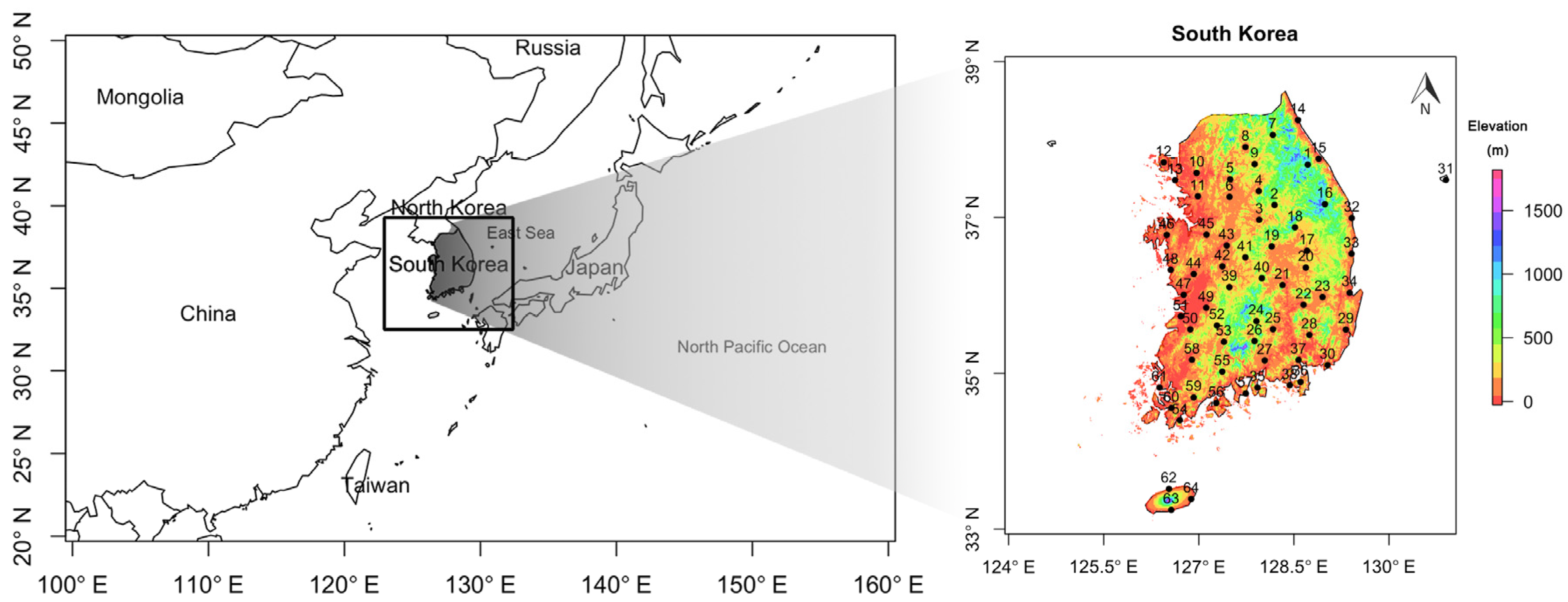
In the current study, an annual maximum (AM) rainfall series of eleven rainfall durations (1 h, 2 h, 3 h, 4 h, 6 h, 12 h, 18 h, 24 h, 48h, 72 h, and 168 h) at 64 weather stations are employed. The area for one rainfall observation station is about 1566 km2. The stations that have more than a 30-year record are selected for analysis. The hourly precipitation data used in the current study are collected from Korea Meteorological Administration (KMA) data base. The location of the weather stations is illustrated in Figure 1, and Table 1 presents their information such as station name, record length, and elevation.
For strict comparative analysis, the temporal series should be done during the same period. To obtain more stable and reliable results of the analysis, all available data for each station are employed in the analyses. For the data employed in this study, the start year of the data is little different for each weather station. However, the end year of data is the same for all employed station (end year of data is 2016). The results of analyses can be employed in comparative analysis in this study.
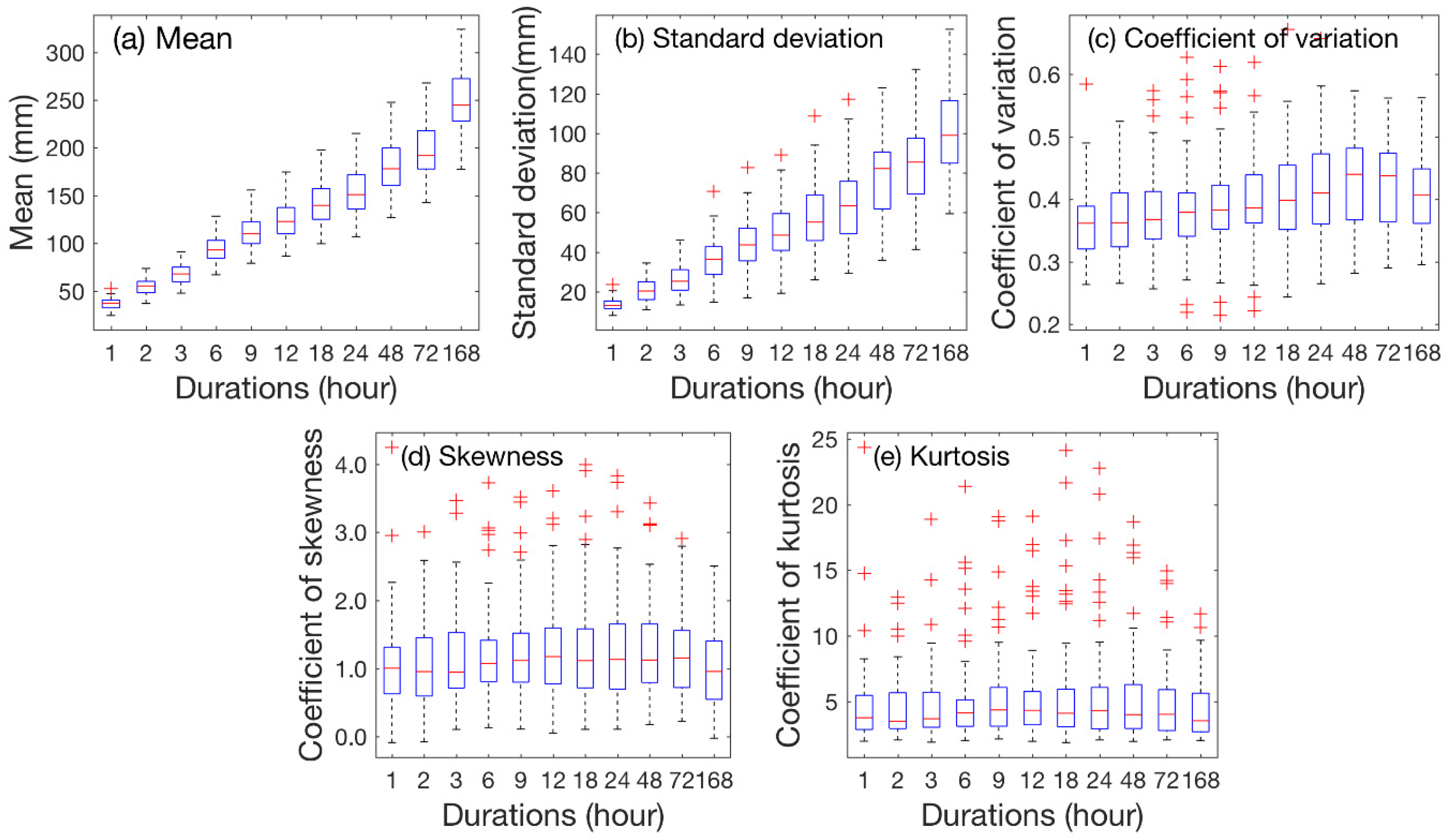
To examine the statistical characteristics of the AM series of South Korea, basic statistics that have been calculated using the AM series for all of the stations are presented in Figure 2. These basic statistics include the mean, the standard deviation, the coefficient of variation (CV), the coefficient of skewness (CS), and the coefficient of kurtosis (CK). The median of the mean estimates increases as the duration becomes longer. This tendency is also observed in the variance of the mean estimates. It is observed in Figure 2c that the median of the CV estimates changes with the duration. The median of the CV estimates increases through 72 h (excluding 168 h) as the duration becomes longer. However, the differences in the median of the CV estimates are small. The variance of the CV estimates varies strongly with the duration. The median and variance of the estimates of the CS and the CK are almost consistent with the durations. The AM series of South Korea display consistent estimates of the CS and the CK for different durations. Since the CS and CK represent the behavior of the right tail of the probability distribution that governs the characteristics of extreme events, the extreme rainfall events of South Korea may have similar distributional characteristics. However, the statistical characteristics of the AM series corresponding to the different durations may differ, due to the discrepancies in the estimates of the mean and the CV.
3. Method
3.1. Block Bootstrap-Based Mann-Kendall Test
The MK test is the one of most popular trend tests because it is simple and non-parametric. The results of the MK trend test are affected by serial correlation in the time series. When positive serial correlation exists within a time series, the possibility that the null hypothesis (i.e., that no trend exists) will be rejected when the null hypothesis is actually true increases [37,38]. Completely independent data sets are difficult to find, due to the presence of external factors that impact the generation of the target data. To overcome these drawbacks, a large number of studies have suggested various modified versions of the MK test for use in the field of hydro-meteorology [39,40,41,42]. The block bootstrap-based MK (BBS-MK) test, which is a modified version of the MK test, was suggested by Khaliq et al. [43]. The performance of the BBS-MK test is comparable to other modified versions of the MK test, and it is simpler and more efficient than these other methods [42].
The procedure used in applying the BBS-MK test is as follows:
- (1)
- Estimate the test statistic S of the MK from the original time series. The test statistic S is given as follows:where and are the sequential data values, and n is the total number of observations in the time series. A positive value of test statistic S indicates an increasing trend, whereas a negative value of this quantity indicates a decreasing trend.
- (2)
- Estimate the number of significant contiguous autocorrelations k. When the autocorrelation is smaller than 5% significant level, the lag of the autocorrelation becomes k.
- (3)
- Resample the original time series a large number of times using blocks of size k + g.
- (4)
- Estimate the test statistic S for each simulated sample to produce a simulated distribution of the test statistic S.
- (5)
- Estimate the significance (p-value) of the test statistic S estimated in Step 1 using the simulated distribution from Step 3.
In this study, 2000 simulated sample sets are resampled from the original data set. Svensson et al. [44] reported that this number leads to stable estimates of the significance in trend tests using simulation methods. Additionally, the optimum value of g is estimated by trial and error. To find the optimum g value, mean and autocorrelation of the observation and the resampled data are computed. The relative absolute error between the observation and resampled data for g from one to one-quarter of sample size computed based on the mean and autocorrelation estimates. The g value giving the smallest relative error is employed as the optimum g value. A detailed method for finding optimum values of g is described in Khaliq et al. [43] and Önöz and Bayazit [42].
3.2. Modified Version of Mann-Kendall Test
Detecting appropriately the trend in the data having serial correlation and small sample size is difficult. To obtain reliable results of trend detection, modified version of Mann-Kendall (modified MK) test adapted by Yue and Wang [45] is employed in the current study. In the modified MK test, the autocorrelation in the data series is taken into account by modifying the variance of the test statics (S). The procedure of the modified MK test is described as below.
Mann [46] and Kendall [47] state that when n is larger than eight the statistic S is approximately normally distributed with the variance given by:
where is the number of ties of extent l. The standard MK statistic Z is computed by Equation (3)
The standard MK statistic Z follows the standard normal distribution under the null hypothesis of no trend. In the modified MK test, the variance of the test statistics V(S) is corrected by multiplying the correction factor (CF) for taking into consideration serial correlation in the data. Equation (4) presents the corrected variance of test statistics.
where is the lag-i serial correlation coefficient from the detrended data or rank of the detrended data. In the current study, the trend in the original data are removed by the Theil-Sen approach as recommend by Hamed and Rao [39] and Blain [48]. The Equations (5) were given by Matalas and Langbein [49] and Bayley and Hammersley [50]. The standard Mk statistic in the modified MK test is defined by Equation (6).
3.3. Scaling Property of Extreme Rainfall Events
Scale invariance is often interpreted as a synonym for other terms such as “self-similar”, “automodal”, and “scaling” [51]. Scale invariance is produced by laws that do not change if the scale of a random variable is multiplied by a scale function. Hence, scale invariance can be expressed by Equation (7). Let and be time series of AM rainfall corresponding to durations and 1, respectively.
where indicates the scaling exponent, and represents the sense of equality of probability distributions. If the wide sense simple scaling holds, it implies that the moments of the AM series for different durations have a relationship that is similar to that presented in Equation (2) [51,52,53]. The scaling relationship of the moments of the AM series can be defined by Equation (8) or (9).
Log of raw moments ( and ) are computed for the given durations () and different order of moment () The scaling exponent () is estimated using the computed log of raw moments by the ordinary least square method. The GEV distribution is widely employed in the modeling of extremes [54,55,56,57,58,59,60,61,62,63,64]. Additionally, the GEV distribution has been used for modeling extreme rainfall events in many studies [65,66,67,68]. The cumulative distribution function (CDF) of the GEV distribution is given by Equation (10).
where , , and are the location, scale, and shape parameters, respectively.
The GEV simple scaling framework has been employed for modeling extreme rainfall intensity by Nguyen et al. [53] and Bougadis and Adamowski [69]. Borga et al. [70] used a Gumbel distribution, which is a special case of the GEV distribution, in the simple scaling framework. Combining Equation (10) with Equation (8) yields the GEV simple scaling framework. In this framework, the location and scale parameters of the GEV distribution change as the duration changes. Their relationships are expressed in Equation (11).
The durations ( and 1) in Equation (6) can take any positive value. For example, if the parameters of the GEV distribution for a 12-h AM series are known, the parameters of the GEV distribution for the corresponding 24-h AM series can be estimated using and . As shown in the previous equation, only the scaling exponent is an unknown parameter. Because the scaling exponent governs the statistical relationship among the AM series of different durations, the scaling exponent represents a key indicator of the temporal structure of extreme rainfall events. Therefore, the scaling exponent is used as an index to represent the temporal structure of extreme rainfall events in this study.
4. Application
To examine the trends in extreme rainfall events in South Korea, the trends in AM series of eleven different durations are examined using the BBS-MK test with a significance level of 5%. The results of the BBS-MK test are subsequently displayed on maps to permit investigation of the spatial characteristics of the trends in the AM series. Since extreme rainfall events in South Korea usually occur during the rainy season, the monthly AM series during the rainy season may display trends, and these trends may differ from those seen in the annual AM series. Investigating the interannual variability of extreme rainfall events is important in water resource management, especially in the mitigation and prevention of floods. Hence, trends in the monthly AM series from May to October including the rainy season are investigated in this study. Additionally, the trend detection results are displayed on maps to permit investigation of the spatial characteristics of trends in the monthly AM series during the rainy season.
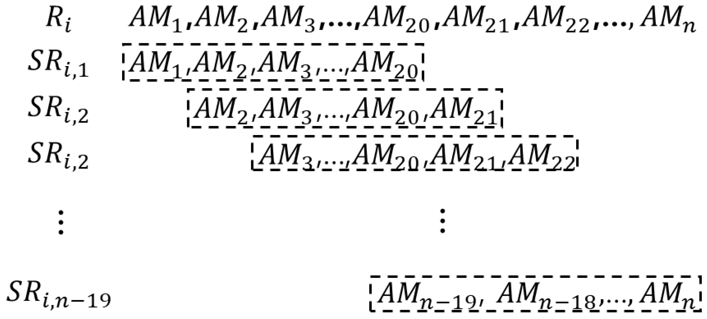
Serial data are needed to perform the BBS-MK trend test. However, a single scaling exponent can be computed for a given data series. Thus, time series of scaling exponent estimates must be calculated. In this study, 20-year moving windows are used to extract subsamples () of the AM series from the whole AM series (), and the scaling exponents of the subsamples are estimated. The methodology used to extract the subsamples is displayed in Figure 3.
Trends in the scaling exponent estimates derived from series of subsamples () on an annual and a monthly basis are detected. The time series of scaling exponent estimates contain strong autocorrelation, due to overlaps in the periods used to create the subsamples from the AM series; thus, conventional trend tests, such as the MK test and the t-test, may not detect the true trends in these data series. Since the BBS-MK trend test accounts for autocorrelation, the BBS-MK test is applied to the time series of scaling exponent estimates in this study. The results of the BBS-MK test are displayed on maps and analyzed to enable assessment of the spatial pattern of the temporal structure of extreme rainfall in South Korea.
5. Results
5.1. Trends in Time Series of Annual Maximum Rainfall
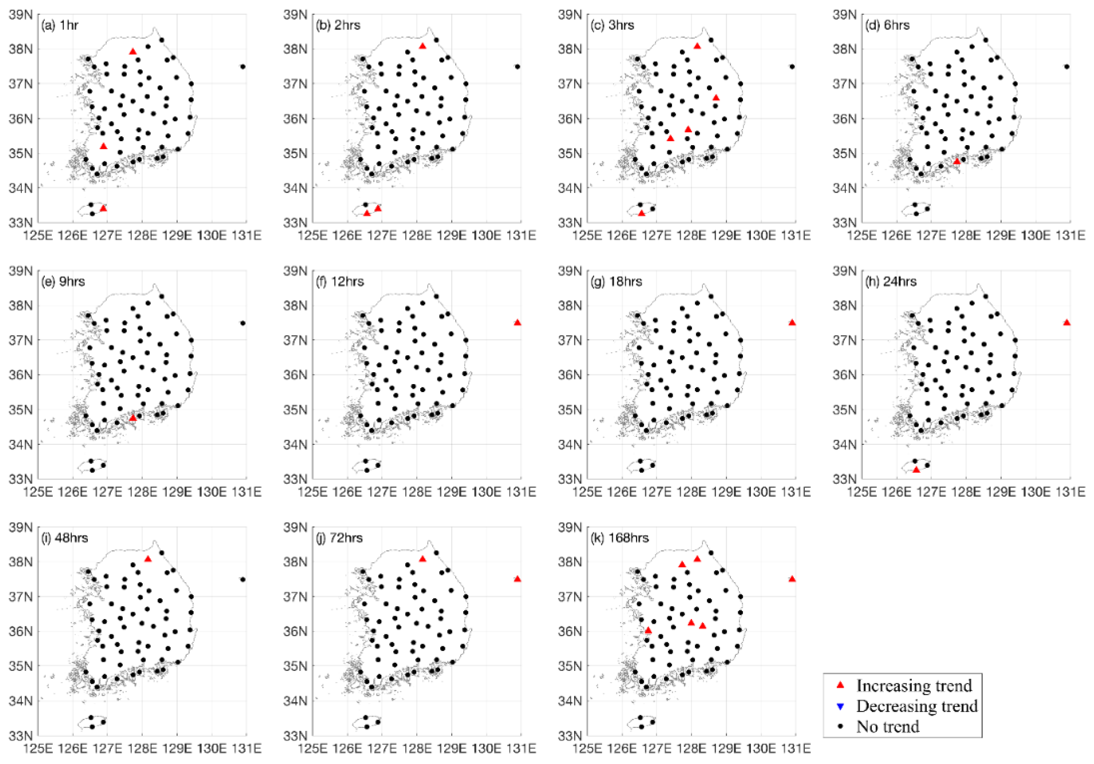
The spatial distribution of the BBS-MK test results for AM series of eleven durations on an annual basis is presented in Figure 4. Many of the studied stations display no significant trends in the AM series for any of the durations investigated here. Significant trends are detected at a small number of stations. All of the detected trends are an increasing trend. The detected trends contain no spatial pattern.
For the May AM series for durations ranging from 1 h to 168 h, the AM series of many of the employed stations display no significant trends. None of the May AM series from the employed stations contain trends for the long durations (from 18 h to 168 h), whereas significant increasing and decreasing trends are detected at some stations for shorter durations (from 1 h to 12 h). For the June AM series for durations of 1 h to 168 h, the AM series of some of the studied stations display significant increasing and decreasing trends. None of the AM series from the studied stations with a duration of 168 h display a significant trend. Decreasing trends are noted in the AM series from the southern region, unlike the results of the trend test in May. The July–October AM series have no significant trends at most of the employed stations. Significant trends are sporadically detected at a few stations and for a few durations. These results indicate that there are no statistically strong trends in the monthly July–October AM series. The results of the BBS-MK test of July to October AM series for durations ranging from 1 h to 168 h are presented in Supplementary Materials.
5.2. Trends in Temporal Structure of the Time Series of Annual Maximum Rainfall
The scaling exponent of the AM series and their standard errors are computed and presented in Table 2. To investigate the uncertainty of scaling exponent estimation, the bootstrapping method is employed. The detailed procedure of the employed bootstrapping method is described in the supplementary material. Based on the standard deviations of the scaling exponents, the differences among the scaling exponents at different stations are large. It is found that the distributions of the scaling exponents are non-Gaussian distribution. Hence, the standard deviations may be improper to represent the uncertainty of the scaling exponent estimation. Scaling exponents corresponding to 2.5 and 97.5 percentiles from the scaling exponent estimates of the resampled data are found. Based on the scaling exponent corresponding to the 2.5 and 97.5 percentiles, the differences among scaling exponents at stations also are large. Additionally, two sample t-test for unequal variances is performed to investigate the difference between mean estimates of scaling exponents. Based on t-test results, mean estimates of scaling exponents at the thirty-four stations are significant different of any other stations based on 5% significant level. Thirty stations have one to three stations that have the similar mean estimates. The results of the t-test are presented in supplementary material. Hence, it can be inferred that the scaling exponent estimates at different stations are dissimilar.
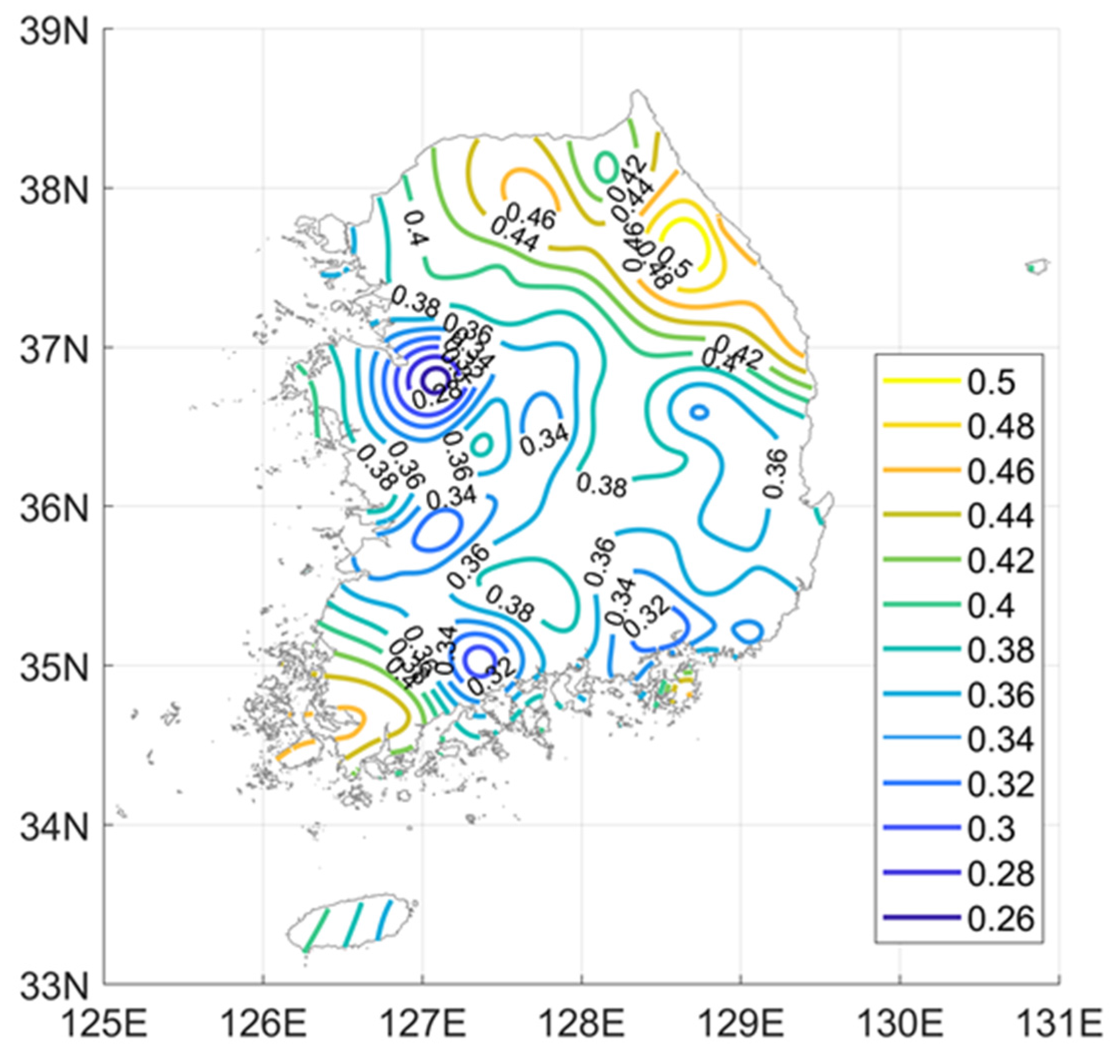
Figure 5 presents a contour map of scaling exponent estimates for the AM series of South Korea. The contour lines show that the scaling exponent estimates of the AM series in South Korea range from 0.25 to 0.5. The scaling exponent estimates in the inland part of the country are approximately 0.35. These results indicate that the temporal structures of the AM series in the inland part of the country are consistent. Large values (greater than 0.45) of the scaling exponents are observed in the northeast, whereas small values (smaller than 0.3) of the scaling exponents are observed in the east. A large value of the scaling exponent means that there is a large and statistical difference between AM events with short and long durations. Hence, the statistical characteristics of the AM series with short and long durations are dissimilar in the northeast. Large variability is observed in the spatial distribution of the scaling exponent estimates; for an example, compare the scaling exponents in the northeastern and eastern areas. These results indicate that the temporal structure of the extreme rainfall events in South Korea displays substantial variability.
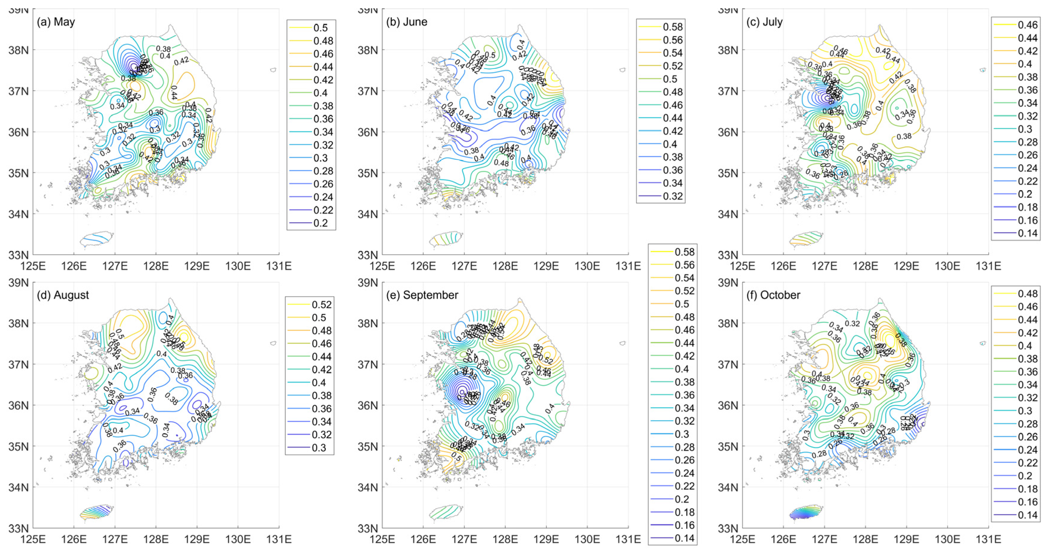
Figure 6 presents contour maps of the scaling exponent estimates for the monthly AM series of South Korea during the rainy season. The variations in the scaling exponent estimates for May, June, July, September, and October are larger than the annual variations in the scaling exponent estimates. As shown in Figure 6a, the scaling exponent estimates of the May AM series range from 0.2 to 0.45. A large variation in the scaling exponent estimates is observed in Figure 6a. The scaling exponent estimates in the coastal areas are larger than the estimates in the inland part of the country. The scaling exponent estimates in the coastal areas (i.e., the northeastern and southwestern areas) in June are large. In July and August, the scaling exponent estimates in the north are larger than those in the southern areas. Very small scaling exponent estimates are observed in the northwest in July and September; moreover, similarly small values can be observed in the same areas in Figure 5. The spatial distribution of the scaling exponent estimates during the employed months in the rainy season displays no dominant tendency. The spatial distributions of the scaling exponents for each month are dissimilar. These results imply that the interannual variability in extreme rainfall events in South Korea is large, especially in terms of the temporal structure of extreme rainfall events.
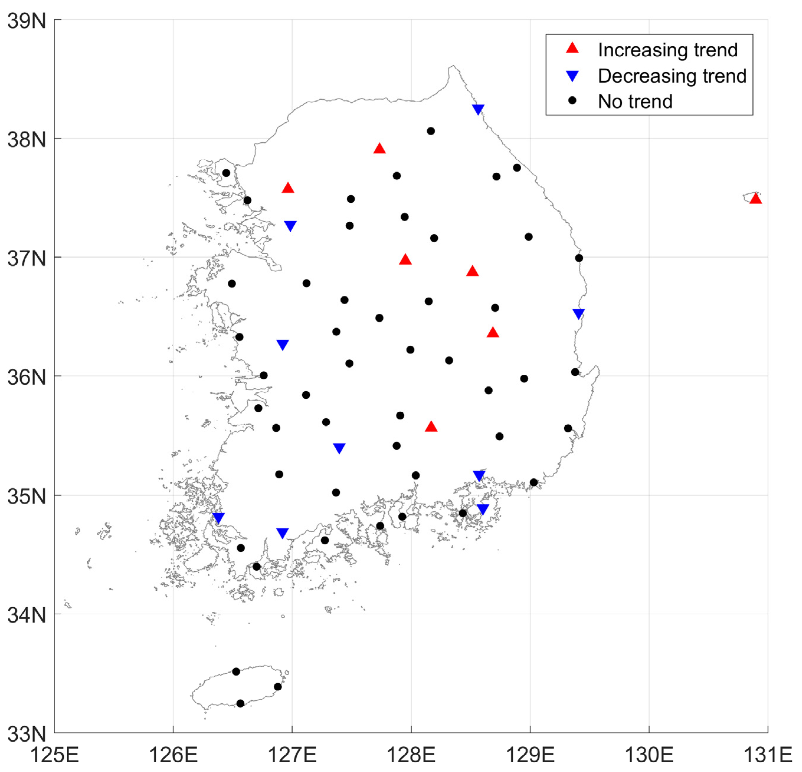
The results of the trend tests that consist of series of scaling exponent estimates for the subsamples of the AM series on an annual basis are shown as maps in Figure 7. The k values used in this study for the series of scaling exponents based on AM series ranges from 0 to 7. Mean of k values is 3. The g values range from 0 to 8 and their mean is 3. The block size (k + g) ranges from 2 to 9 and mean of the block size is 6. Önöz and Bayazit [42] suggested that optimal block size is 5 when sample size 25 and higher autocorrelation. In their study, performance of the BBS-MK test with block size = 6 is almost same as the performance with block size = 5. Hence, the selection of block size in this study is reasonable to carry out the BBS-MK test. Sample sizes of the employed scaling exponent series are relatively small. Thus, the BBS-MK test may not successfully provide reliable results of the trend detection at some stations. To attenuate and avoid the misdetection of trends, the modified MK test is additionally carried out. The stations that two methods detected the trend are considered as the scaling exponent series have trends. Based on the results of the trend tests, significant trends are observed in the subsamples of the AM series at many of the stations, unlike the results of the trend test applied to the AM series. Decreasing trends are observed at many stations located in the coastal areas, particularly the southwest, whereas increasing trends are observed in the inland part of the country. Hence, the differences in the statistical characteristics of the AM series for different durations in the coastal areas are becoming smaller because the scaling exponents are decreasing over time. Moreover, the variability in the AM series of different durations in the inland part of the country increases over time.
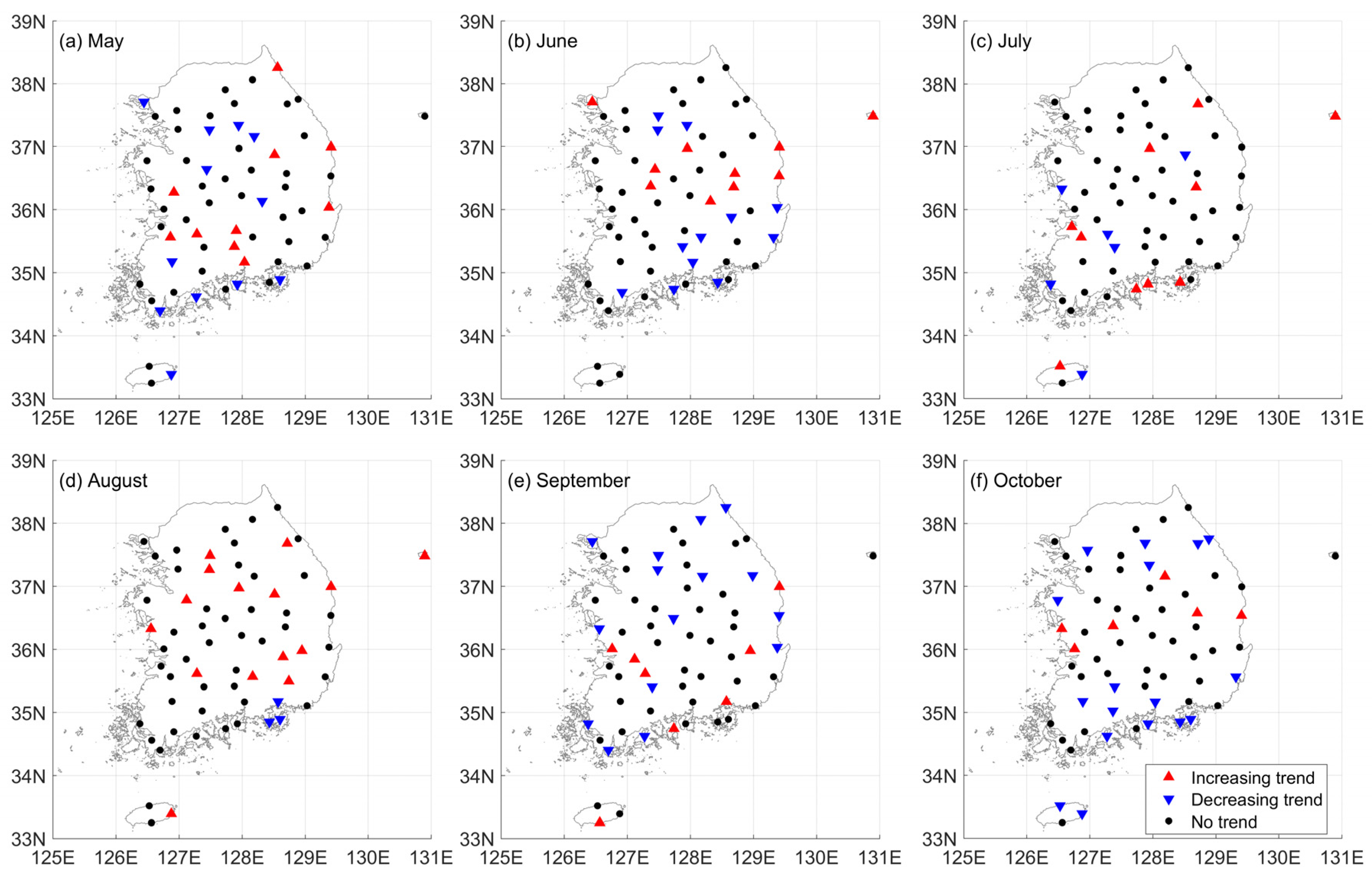
Figure 8 presents the results of the trend tests in terms of time series of scaling exponent estimates for the subsamples of the AM series on a monthly basis in the rainy season. The spatial distributions of the trends in the time series of scaling exponent estimates differ by month. In the time series of scaling exponent estimates derived from the May AM series, decreasing trends are observed in the southern and northwestern areas, and increasing trends are observed in the west-central and eastern areas. The scaling exponents obtained for many stations in the southern area, as well as at four stations in the north, for June display decreasing trends. Increasing trends are observed for many stations in the central area of South Korea. For the July scaling exponent estimates, significant trends are detected at the smallest number of stations.
Decreasing trends in the time series of scaling exponent estimates of the August AM series are observed in the southern coastal area, and many of the stations in the other parts of the country show increasing trends. From these results, it can be inferred that the differences in the statistical characteristics of the August AM series of different durations are becoming larger over time. The scaling exponents at many stations in the north show decreasing trends for September. In the southern area, decreasing and increasing trends are sporadically observed in the time series of scaling exponent estimates for September. The scaling exponents at many of the stations in the southern coastal area and the northern area display decreasing trends. Additionally, increasing trends in the scaling exponents for October are observed at six stations located in the central area.
6. Discussion
6.1. Characteristics of Spatial and Temporal Structure of Extreme Rainfall Trends in South Korea
No trends are evident in the AM series of any of the durations examined at most of the employed stations. Additionally, no station consistently displays a trend for all of the durations examined. For the AM series of each month (May to October), there are statistically significant trends at a few stations. Additionally, no station consistently displays a trend for all of the durations examined. All of the detected trends in the annual and monthly AM series are an increasing trend. Thus, although the magnitude of extreme rainfall in South Korea is increasing over time, the changes are very small, and the temporal and spatial structures display inconsistent trends.
The temporal structure of extreme rainfall events can be represented by the scaling exponent. For example, when the scaling exponent derived from AM series is small, the differences in the location parameters of the AM series with different durations are small. Thus, at stations associated with small scaling exponents, the differences among the statistical properties of the AM series with different durations are small, and vice versa. The scaling exponent estimates derived from the AM series in South Korea differ strongly, based on the locations of the stations. For instance, the scaling exponents in the northeast are greater than 0.4, whereas the scaling exponents in the northwest are less than 0.3. The scaling exponents for the AM series of each month are spatially inhomogeneous. Moreover, their spatial distributions are dissimilar. Thus, the spatial distribution of the temporal structure associated with extreme rainfall in South Korea displays large variability. In addition, the interannual variability in the temporal structure of extreme rainfall in South Korea is very large.
The cause of spatial and temporal variation in various hydro-meteorological extremes is very complicated. Particularly, spatial and temporal variation of extreme rainfalls in South Korea are influenced by mountainous terrain, monsoon, and typhoon. Therefore, it is very difficult to analyze spatio-temporal variation in South Korea [11,71]. Chang and Kwon [72] analyzed spatial variation of precipitation trends monthly during summer (rainy season) in South Korea using daily precipitation data between 1973 and 2005. They reported that spatial variations of the precipitation trends in summer was very different in each month. They discussed that it is likely to have some connection with large-scale atmospheric circulation, variation of sea surface temperature and geographic features. Consequently, amount and intensity of summer rainfall in South Korea have changed with time and space. They mentioned that these variations are the temporal redistribution of summer rainfall occurred in South Korea caused by climate change.
In this study, we also confirmed the temporal and spatial redistribution from the various contour maps of the scaling exponent estimate for each month. The scaling exponent estimates have changed with time and space during the rainy season. The variations of scaling exponents between June and July are most likely to be caused a seasonal rain front (i.e., monsoon) movement. In addition, spatial changes in the scaling exponent estimates from September and October are more likely to be due to typhoons. Spatial and temporal variations observed in this study may be due to hydro-meteorological phenomena such as monsoon and typhoon which are main contributors of extreme rainfalls in South Korea. Occurring time and intensity of these phenomena are different for each year. Therefore, the spatial distribution of the scaling exponents for each month are not consistent.
Scaling exponent estimates and scaling properties have been used to derive regional IDF curves [70,73,74,75]. Yu, Yang and Lin [73] carried out a regionalization to identify homogeneous regions based on the scaling exponent. Additionally, since the scaling exponent represents the temporal structure of extreme rainfall events, it may be possible to use the scaling exponent to cluster stations that are homogeneous in terms of their extreme rainfall events for use in regional IDF analyses. Hence, the regionalization of the extreme rainfall events in South Korea should be performed with care, due to the large spatial and interannual variability in the temporal structure of the extreme rainfall events.
While the AM series at a small number of stations display statistically significant trends, significant trends are detected at many stations when the time series of scaling exponent estimates are used (see Figure 4 and Figure 7). Furthermore, both increasing and decreasing trends are detected in the time series of scaling exponent estimates, unlike the results of applying the trend analysis to the AM series. Even though the AM series of a small number of stations display significant trends, the scaling exponents present nonstationarity. These results indicate that applying trend analysis to extreme rainfall events is insufficient to check the nonstationarity associated with extreme events. The results of applying the BBS-MK test to the AM series of South Korea show that the AM series may contain very weak increasing trends; the AM series at most of the employed stations can be considered to be stationary, and the AM series at a few stations display increasing trends. However, the temporal structures of the AM series at many stations in South Korea can be considered to reflect nonstationary conditions, based on the results of applying the trend tests to time series of scaling exponent estimates. Hence, the detailed trends of the extreme rainfall events and their temporal structures should be assessed to investigate the nonstationarity in the extreme rainfall events.
Since the trends in the time series of scaling exponent estimates may influence the regionalization, the homogeneous regions clustered using current data will change in the future. These trends should be taken into consideration in deriving a regional IDF curve for South Korea. These trends should also be considered for the nonstationary IDF curves of the extreme rainfall events in South Korea. Conventional nonstationary IDF curves assume that the temporal structure of extreme rainfall events is constant over time [76,77]. For example, Cheng and AghaKouchak [78] employed a nonstationary GEV distribution with a time-varying location parameter to model a nonstationary IDF curve. They fitted the nonstationary GEV distribution for each duration examined, and their study provided an IDF curve for extreme rainfall events in the U.S. Sarhadi and Soulis [79] modeled a nonstationary IDF curve using the nonstationary GEV distribution with time-varying location and scale parameters. However, the temporal structure of the extreme rainfall events of South Korea change, although there is no trend in the mean of extreme rainfall events. Thus, the conventional approach used in modeling nonstationary IDF curves, which involves the use of the nonstationary GEV distribution with a covariate, may not properly represent extreme rainfall in South Korea.
The model used to derive the nonstationary IDF curve for South Korea should account for trends in temporal structure. For example, the scaling exponent in Equation (5) can be allowed to vary with time, instead of the location or scale parameters of the GEV distribution. Employing the scaling exponent as a time-varying parameter in the GEV simple scaling framework may be an adequate parameterization for the representative model of the nonstationary IDF curve in South Korea, since significant trends are not detected in the AM series at many stations. In cases where a trend exists in the AM series at a given station, the location parameter and the scaling exponent can be permitted to vary with time.
6.2. Limitation of the Employed Methodology
The scaling exponent series have the serial correlations. Due to the serial correlation, the trend tests employed in the current study consider the serial correlation in the data. In the current study, results of two trend tests are very similar but not the same. The methods to derive the distribution of Mann-Kendal statistics are different in two employed tests. The modified version of Mann-Kendall test considered that the distribution of Mann-Kendal statistics follows the normal distribution. This test takes consideration of the influence of the serial correlation in the trend detection by modifying the variance of the mean. In the BBS-MK test, the distribution of Mann-Kendall statistics may not be the same as the normal distribution since the distribution is obtained by the block bootstrapping method. The distribution of Mann-Kendall statistics in the BBS-MK test may be different depending on the data.
Both tests have pros and cons. The subjective decisions are not required in the modified version of the Mann-Kendall test. For the large sample size, the distribution of the Mann-Kendall statistics follows the normal distribution [39]. However, in small sample size, the distribution of the Mann-Kendall statistics may not exactly follow the normal distribution [80]. In the case of small sample size, the modified version of Mann-Kendall test can lead to low power to detect trends due to the normal distribution assumption. The BBS-MK test derives the distribution the distribution of the Mann-Kendall statistics by the block bootstrapping method. The shape of the Mann-Kendall statistic distribution for various sample size and data may be close to the distribution of the Mann-Kendall statistic in population. However, in the BBS-MK test, obtaining an accurate distribution shape from bootstrapping is difficult due to difficulty in the selection of an optimal block size.
According to the results of the Mann-Kendall test, some stations where the BBS-MK test detected trends did not trend. Some stations where the modified version of the Mann-Kendall test detected trends did not have trends based on the results of the BBS-MK test. These results may come from the issue of small sample size. Basically, the results of two tests should be similar because both tests attempt to detect a trend in the data. If the sample size is very large, two different tests may provide the same results. The small sample size is the limitation of the employed methodology in the current study. Thus, to attenuate and avoid the probability to obtain inappropriate results of trend detection from the small sample size, a number of trend tests should be employed. The application of a number of trend tests leads to more reliable results for trend detection in the serially correlated data with the small sample size. Although the results of the current study may not be the perfect results due to the limitation, the results can provide the glance to the trends in the spatial and temporal structure of extreme rainfall in South Korea.
7. Conclusions
The spatial and temporal structures of extreme rainfall trends in South Korea are investigated in this study. The trends in the annual and monthly AM series are detected, and their spatial distributions are analyzed. The scaling exponent is employed as an index to represent the temporal structure. The temporal structure of extreme rainfall events is calculated and shown on maps. Subsequently, the BBS-MK and modified MK tests are employed for the time series of scaling exponent estimates of the AM series on the annual and monthly basis. The results of the BBS-MK and modified MK tests are displayed on maps, and their characteristics are analyzed. In this study, we reach the following conclusions:
- Significant trends are detected at a small number of stations, while no significant trends in extreme rainfall events can be found at many stations for the durations examined. Significant trends are sporadically detected at a few stations and for a few durations. There is no spatial pattern of the detected trends.
- There is large variability in the temporal structures of the extreme rainfall events. The scaling exponent estimates of the AM series in South Korea range from 0.25 to 0.5. The scaling exponent estimates in the inland part of the country are approximately 0.35. Large values of the scaling exponent are observed in the northeast, and small values of the scaling exponent are observed in the northeast. Additionally, the interannual variability in the temporal structure of the AM series is very large during the rainy season. The variations in the scaling exponent estimates during the rainy season are larger than those inferred using annual data. The spatial distribution of the scaling exponent estimates during the rainy season displays no dominant tendency. The spatial distributions of the scaling exponents for each month are dissimilar.
- Significant trends exist in the temporal structures of extreme rainfall events at many stations in South Korea. Decreasing trends are observed at many stations located in the coastal area, particularly in the southwest, whereas increasing trends are observed in the inland part of the country. The variability in the AM series with different durations in the inland part of the country is increasing over time. Additionally, the interannual variability in the trends in the temporal structure of extreme rainfall in South Korea is large. The spatial distributions of the trends for the time series of scaling exponent estimates differ by month.
Modeling of IDF curves using regionalization based on the scaling exponents associated with extreme rainfall events in South Korea would be a fruitful topic for further studies. Additionally, nonstationary IDF curves that account for trends in the temporal structure of extreme rainfall in South Korea should be studied in the future.
Supplementary Materials
The following are available online at www.mdpi.com/2073-4441/9/10/809/s1, Figure S1: The BBS-MK test results of AM series on May for 1-hour to 168-hour durations at 5% significant level, Figure S2: The BBS-MK test results of AM series on June for 1-hour to 168-hour durations at 5% significant level, Figure S3: The BBS-MK test results of AM series on July for all employed durations at 5% significant level, Figure S4: The BBS-MK test results of AM series on August for all employed durations at 5% significant level, Figure S5: The BBS-MK test results of AM series on September for all employed durations at 5% significant level, Figure S6: The BBS-MK test results of AM series on October for all employed durations at 5% significant level, Table S1. Results of t-test between the scaling exponents for two of any employed stations.
Acknowledgments
This work is supported by the Korea Agency for Infrastructure Technology Advancement (KAIA) grant funded by the Ministry of Land, Infrastructure and Transport (Grant 17AWMP-B083066-04).
Author Contributions
For research articles with several authors, a short paragraph specifying their individual contributions must be provided. The following statements should be used “J.-Y. Shin and J.-H. Heo conceived and designed the experiments; Y. Jung performed the experiments; Y. Jung and J.-Y. Shin analyzed the data; J.-Y. Shin and H. Ahn contributed reagents/materials/analysis tools; Y. Jung and J.-Y. Shin wrote the paper.” Authorship must be limited to those who have contributed substantially to the work reported.
Conflicts of Interest
The authors declare no conflict of interest.
References
- Balling, R.C., Jr.; Cerveny, R.S. Compilation and discussion of trends in severe storms in the United States: Popular perception v. Climate reality. Nat. Hazards 2003, 29, 103–112. [Google Scholar] [CrossRef]
- Garcia, J.A.; Gallego, M.C.; Serrano, A.; Vaquero, J.M. Trends in block-seasonal extreme rainfall over the Iberian Peninsula in the second half of the twentieth century. J. Clim. 2007, 20, 113–130. [Google Scholar] [CrossRef]
- Modarres, R.; da Silva, V.P.R. Rainfall trends in arid and semi-arid regions of Iran. J. Arid Environ. 2007, 70, 344–355. [Google Scholar] [CrossRef]
- Ntegeka, V.; Willems, P. Trends and multidecadal oscillations in rainfall extremes, based on a more than 100-year time series of 10 min rainfall intensities at Uccle, Belgium. Water Resour. Res. 2008, 44. [Google Scholar] [CrossRef]
- Aryal, S.K.; Bates, B.C.; Campbell, E.P.; Li, Y.; Palmer, M.J.; Viney, N.R. Characterizing and modeling temporal and spatial trends in rainfall extremes. J. Hydrometeorol. 2009, 10, 241–253. [Google Scholar] [CrossRef]
- Acero, F.J.; García, J.A.; Gallego, M.C. Peaks-over-threshold study of trends in extreme rainfall over the Iberian Peninsula. J. Clim. 2010, 24, 1089–1105. [Google Scholar] [CrossRef]
- McAfee, S.A.; Guentchev, G.; Eischeid, J.K. Reconciling precipitation trends in Alaska: 1. Station-based analyses. J. Geophys. Res.: Atmos. 2013, 118, 7523–7541. [Google Scholar] [CrossRef]
- Sarr, M.A.; Zoromé, M.; Seidou, O.; Bryant, C.R.; Gachon, P. Recent trends in selected extreme precipitation indices in senegal—A changepoint approach. J. Hydrol. 2013, 505, 326–334. [Google Scholar] [CrossRef]
- Ye, Z.; Li, Z. Spatiotemporal variability and trends of extreme precipitation in the huaihe river basin, a climatic transitional zone in east China. Adv. Meteorol. 2017, 2017, 1–15. [Google Scholar]
- Zwiers, F.W.; Kharin, V.V. Changes in the extremes of the climate simulated by CCC GCM2 under CO2 doubling. J. Clim. 1998, 11, 2200–2222. [Google Scholar] [CrossRef]
- Boo, K.O.; Kwon, W.T.; Baek, H.J. Change of extreme events of temperature and precipitation over Korea using regional projection of future climate change. Geophys. Res. Lett. 2006, 33. [Google Scholar] [CrossRef]
- Kay, A.L.; Reynard, N.S.; Jones, R.G. RCM rainfall for UK flood frequency estimation. I. Method and validation. J. Hydrol. 2006, 318, 151–162. [Google Scholar] [CrossRef]
- Kay, A.L.; Jones, R.G.; Reynard, N.S. RCM rainfall for UK flood frequency estimation. II. Climate change results. J. Hydrol. 2006, 318, 163–172. [Google Scholar] [CrossRef]
- Wang, D.; Hagen, S.C.; Alizad, K. Climate change impact and uncertainty analysis of extreme rainfall events in the apalachicola river basin, Florida. J. Hydrol. 2013, 480, 125–135. [Google Scholar] [CrossRef]
- Shahabul Alam, M.; Elshorbagy, A. Quantification of the climate change-induced variations in intensity–duration–frequency curves in the canadian prairies. J. Hydrol. 2015, 527, 990–1005. [Google Scholar] [CrossRef]
- Lee, O.; Park, Y.; Kim, E.S.; Kim, S. Projection of korean probable maximum precipitation under future climate change scenarios. Adv. Meteorol. 2016, 2016, 1–16. [Google Scholar] [CrossRef]
- Langousis, A.; Veneziano, D.; Furcolo, P.; Lepore, C. Multifractal rainfall extremes: Theoretical analysis and practical estimation. Chaos Solitons Fractals 2009, 39, 1182–1194. [Google Scholar] [CrossRef]
- Rodríguez, R.; Navarro, X.; Casas, M.C.; Ribalaygua, J.; Russo, B.; Pouget, L.; Redaño, A. Influence of climate change on idf curves for the metropolitan area of Barcelona (Spain). Int. J. Climatol. 2014, 34, 643–654. [Google Scholar] [CrossRef] [Green Version]
- Bairwa, A.K.; Khosa, R.; Maheswaran, R. Developing intensity duration frequency curves based on scaling theory using linear probability weighted moments: A case study from India. J. Hydrol. 2016, 542, 850–859. [Google Scholar] [CrossRef]
- Ghanmi, H.; Bargaoui, Z.; Mallet, C. Estimation of intensity-duration-frequency relationships according to the property of scale invariance and regionalization analysis in a mediterranean coastal area. J. Hydrol. 2016, 541, 38–49. [Google Scholar] [CrossRef]
- Tan, X.; Gan, T.Y. Multifractality of Canadian precipitation and streamflow. Int. J. Climatol. 2017. [Google Scholar] [CrossRef]
- Menabde, M.; Seed, A.; Pegram, G. A simple scaling model for extreme rainfall. Water Resour. Res. 1999, 35, 335–339. [Google Scholar] [CrossRef]
- Galmarini, S.; Steyn, D.G.; Ainslie, B. The scaling law relating world point-precipitation records to duration. Int. J. Climatol. 2004, 24, 533–546. [Google Scholar] [CrossRef]
- Ceresetti, D.; Molinié, G.; Creutin, J.D. Scaling properties of heavy rainfall at short duration: A regional analysis. Water Resour. Res. 2010, 46. [Google Scholar] [CrossRef]
- Rodríguez-Solà, R.; Casas-Castillo, M.C.; Navarro, X.; Redaño, Á. A study of the scaling properties of rainfall in spain and its appropriateness to generate intensity-duration-frequency curves from daily records. Int. J. Climatol. 2017, 37, 770–780. [Google Scholar] [CrossRef]
- Jung, I.W.; Bae, D.H.; Kim, G. Recent trends of mean and extreme precipitation in Korea. Int. J. Climatol. 2011, 31, 359–370. [Google Scholar] [CrossRef]
- Park, J.-S.; Kang, H.-S.; Lee, Y.S.; Kim, M.-K. Changes in the extreme daily rainfall in South Korea. Int. J. Clim. 2011, 31, 2290–2299. [Google Scholar] [CrossRef]
- Wi, S.; Valdés, J.; Steinschneider, S.; Kim, T.-W. Non-stationary frequency analysis of extreme precipitation in South Korea using peaks-over-threshold and annual maxima. Stoch. Environ. Res. Risk Assess. 2016, 30, 583–606. [Google Scholar] [CrossRef]
- Jung, Y.; Kim, S.; Kim, T.; Heo, J.-H. Rainfall quantile estimation using scaling property in Korea. J. Korea Water Resour. Assoc. 2008, 41, 873–884. [Google Scholar] [CrossRef]
- Kim, J.-Y.; Kwon, H.-H.; Lee, B.-S. A bayesian glm model based regional frequency analysis using scaling properties of extreme rainfalls. J. Korea Soc. Civ. Eng. 2017, 37, 29–41. [Google Scholar] [CrossRef]
- Kang, H.S.; Cha, D.H.; Lee, D.K. Evaluation of the mesoscale model/land surface model (MM5/LSM) coupled model for East Asian summer monsoon simulations. J. Geophys. Res.: Atmos. 2005, 110. [Google Scholar] [CrossRef]
- Baek, H.-J.; Kim, M.-K.; Kwon, W.-T. Observed short- and long-term changes in summer precipitation over South Korea and their links to large-scale circulation anomalies. Int. J. Climatol. 2017, 37, 972–986. [Google Scholar] [CrossRef]
- Im, E.-S.; Ahn, J.-B.; Remedio, A.R.; Kwon, W.-T. Sensitivity of the regional climate of East/Southeast Asia to convective parameterizations in the RegCM3 modelling system. Part 1: Focus on the Korean Peninsula. Int. J. Climatol. 2008, 28, 1861–1877. [Google Scholar] [CrossRef]
- Lau, K.-M.; Li, M.-T. The monsoon of East Asia and its global associations—A survey. Bull. Am. Meteorol. Soc. 1984, 65, 114–125. [Google Scholar] [CrossRef]
- Kim, J.-S.; Jain, S. Precipitation trends over the Korean peninsula: Typhoon-induced changes and a typology for characterizing climate-related risk. Environ. Res. Lett. 2011, 6, 1–6. [Google Scholar] [CrossRef]
- Korea Meteorological Administration (KMA). Typhoon White Book; KMA: Seoul, Korea, 2011; p. 330. [Google Scholar]
- Von Storch, H. Misuses of statistical analysis in climate research. In Analysis of Climate Variability: Applications of Statistical Techniques Proceedings of an Autumn School Organized by the Commission of the European Community on Elba from 30 October to 6 November 1993; von Storch, H., Navarra, A., Eds.; Springer: Berlin/Heidelberg, Germany, 1999; pp. 11–26. [Google Scholar]
- Yue, S.; Pilon, P.; Phinney, B.; Cavadias, G. The influence of autocorrelation on the ability to detect trend in hydrological series. Hydrol. Process. 2002, 16, 1807–1829. [Google Scholar] [CrossRef]
- Hamed, K.H.; Rao, A. A modified mann-kendall trend test for autocorrelated data. J. Hydrol. 1998, 204, 182–196. [Google Scholar] [CrossRef]
- Yue, S.; Wang, C.Y. Applicability of prewhitening to eliminate the influence of serial correlation on the mann-kendall test. Water Resour. Res. 2002, 38, WR000861. [Google Scholar] [CrossRef]
- Yue, S.; Wang, C. The mann-kendall test modified by effective sample size to detect trend in serially correlated hydrological series. Water Resour. Manag. 2004, 18, 201–218. [Google Scholar] [CrossRef]
- Önöz, B.; Bayazit, M. Block bootstrap for mann-kendall trend test of serially dependent data. Hydrol. Process. 2012, 26, 3552–3560. [Google Scholar] [CrossRef]
- Khaliq, M.N.; Ouarda, T.B.M.J.; Gachon, P.; Sushama, L.; St-Hilaire, A. Identification of hydrological trends in the presence of serial and cross correlations: A review of selected methods and their application to annual flow regimes of Canadian rivers. J. Hydrol. 2009, 368, 117–130. [Google Scholar] [CrossRef]
- Svensson, C.; Kundzewicz, W.Z.; Maurer, T. Trend detection in river flow series: 2. Flood and low-flow index series/détection de tendance dans des séries de débit fluvial: 2. Séries d’indices de crue et d’étiage. Hydrol. Sci. J. 2005, 50, 811–824. (In French) [Google Scholar] [CrossRef]
- Yue, S.; Wang, C.Y. Regional streamflow trend detection with consideration of both temporal and spatial correlation. Int. J. Climatol. 2002, 22, 933–946. [Google Scholar] [CrossRef]
- Mann, H.B. Nonparametric tests against trend. Econometrica 1945, 13, 245–259. [Google Scholar] [CrossRef]
- Kendall, M.G. Rank Correlation Methods; Griffin, C., Ed.; Oxford: London, UK, 1948. [Google Scholar]
- Blain, G.C. The modified mann-kendall test: On the performance of three variance correction approaches. Bragantia 2013, 72, 416–425. [Google Scholar] [CrossRef]
- Matalas, N.C.; Langbein, W.B. Information content of the mean. J. Geophys. Res. 1962, 67, 3441–3448. [Google Scholar] [CrossRef]
- Bayley, G.V.; Hammersley, J.M. The “effective” number of independent observations in an autocorrelated time series. J. R. Stat. Soc. 1946, 8, 184–197. [Google Scholar] [CrossRef]
- Gupta, V.K.; Waymire, E. Multiscaling properties of spatial rainfall and river flow distributions. J. Geophys. Res. Atmos. 1990, 95, 1999–2009. [Google Scholar] [CrossRef]
- Burlando, P.; Rosso, R. Scaling and muitiscaling models of depth-duration-frequency curves for storm precipitation. J. Hydrol. 1996, 187, 45–64. [Google Scholar] [CrossRef]
- Nguyen, V.T.V.; Nguyen, T.D.; Wang, H. Regional estimation of short duration rainfall extremes. Water Sci. Technol. 1998, 37, 15–19. [Google Scholar]
- Ahmad, M.I.; Sinclair, C.D.; Spurr, B.D. Assessment of flood frequency models using empirical distribution function statistics. Water Resour. Res. 1988, 24, 1323–1328. [Google Scholar] [CrossRef]
- Farquharson, F.A.K.; Meigh, J.R.; Sutcliffe, J.V. Regional flood frequency analysis in arid and semi-arid areas. J. Hydrol. 1992, 138, 487–501. [Google Scholar] [CrossRef]
- Martins, E.S.; Stedinger, J.R. Generalized maximum-likelihood generalized extreme-value quantile estimators for hydrologic data. Water Resour. Res. 2000, 36, 737–744. [Google Scholar] [CrossRef]
- El-Adlouni, S.; Ouarda, T.B.M.J.; Zhang, X.; Roy, R.; Bobée, B. Generalized maximum likelihood estimators for the nonstationary generalized extreme value model. Water Resour. Res. 2007, 43. [Google Scholar] [CrossRef]
- Heo, J.H.; Kho, Y.W.; Shin, H.; Kim, S.; Kim, T. Regression equations of probability plot correlation coefficient test statistics from several probability distributions. J. Hydrol. 2008, 355, 1–15. [Google Scholar] [CrossRef]
- El-Adlouni, S.; Ouarda, T.B.M.J. Joint bayesian model selection and parameter estimation of the generalized extreme value model with covariates using birth-death markov chain monte carlo. Water Resour. Res. 2009, 45, W06403. [Google Scholar] [CrossRef]
- Heo, J.-H.; Shin, H.; Nam, W.; Om, J.; Jeong, C. Approximation of modified anderson–darling test statistics for extreme value distributions with unknown shape parameter. J. Hydrol. 2013, 499, 41–49. [Google Scholar] [CrossRef]
- Masina, M.; Lamberti, A. A nonstationary analysis for the northern adriatic extreme sea levels. J. Geophys. Res. Ocean 2013, 118, 3999–4016. [Google Scholar] [CrossRef]
- Rahman, A.; Rahman, A.; Zaman, M.; Haddad, K.; Ahsan, A.; Imteaz, M. A study on selection of probability distributions for at-site flood frequency analysis in Australia. Nat. Hazards 2013, 69, 1803–1813. [Google Scholar] [CrossRef]
- Nasri, B.; El Adlouni, S.; Ouarda, T.B. Bayesian estimation for GEV-B-Spline model. Open J. Stat. 2013, 3, 118–128. [Google Scholar] [CrossRef]
- Nguyen, C.C.; Gaume, E.; Payrastre, O. Regional flood frequency analyses involving extraordinary flood events at ungauged sites: Further developments and validations. J. Hydrol. 2014, 508, 385–396. [Google Scholar] [CrossRef]
- Overeem, A.; Buishand, A.; Holleman, I. Rainfall depth-duration-frequency curves and their uncertainties. J. Hydrol. 2008, 348, 124–134. [Google Scholar] [CrossRef]
- Villarini, G. Analyses of annual and seasonal maximum daily rainfall accumulations for Ukraine, Moldova, and Romania. Int. J. Climatol. 2012, 32, 2213–2226. [Google Scholar] [CrossRef]
- Veneziano, D.; Yoon, S. Rainfall extremes, excesses, and intensity-duration-frequency curves: A unified asymptotic framework and new nonasymptotic results based on multifractal measures. Water Resour. Res. 2013, 49, 4320–4334. [Google Scholar] [CrossRef]
- Rulfová, Z.; Buishand, A.; Roth, M.; Kyselý, J. A two-component generalized extreme value distribution for precipitation frequency analysis. J. Hydrol. 2016, 534, 659–668. [Google Scholar] [CrossRef]
- Bougadis, J.; Adamowski, K. Scaling model of a rainfall intensity-duration-frequency relationship. Hydrol. Process. 2006, 20, 3747–3757. [Google Scholar] [CrossRef]
- Borga, M.; Vezzani, C.; Fontana, G.D. Regional rainfall depth–duration–frequency equations for an alpine region. Nat. Hazards 2005, 36, 221–235. [Google Scholar] [CrossRef]
- Im, E.S.; Jung, I.W.; Bae, D.H. The temporal and spatial structures of recent and future trends in extreme indices over Korea from a regional climate projection. Int. J. Climatol. 2011, 31, 72–86. [Google Scholar] [CrossRef]
- Chang, H.; Kwon, W.-T. Spatial variations of summer precipitation trends in South Korea, 1973–2005. Environ. Res. Lett. 2007, 2, 045012. [Google Scholar] [CrossRef]
- Yu, P.-S.; Yang, T.-C.; Lin, C.-S. Regional rainfall intensity formulas based on scaling property of rainfall. J. Hydrol. 2004, 295, 108–123. [Google Scholar] [CrossRef]
- Blanchet, J.; Ceresetti, D.; Molinié, G.; Creutin, J.D. A regional GEV scale-invariant framework for intensity–duration–frequency analysis. J. Hydrol. 2016, 540, 82–95. [Google Scholar] [CrossRef]
- Soltani, S.; Helfi, R.; Almasi, P.; Modarres, R. Regionalization of rainfall intensity-duration-frequency using a simple scaling model. Water Resour. Manag. 2017, 31, 4253–4273. [Google Scholar] [CrossRef]
- Cheng, L.; AghaKouchak, A.; Gilleland, E.; Katz, R. Non-stationary extreme value analysis in a changing climate. Clim. Chang. 2014, 127, 353–369. [Google Scholar] [CrossRef]
- Vasiliades, L.; Galiatsatou, P.; Loukas, A. Nonstationary frequency analysis of annual maximum rainfall using climate covariates. Water Resour. Manag. 2015, 29, 339–358. [Google Scholar] [CrossRef]
- Cheng, L.; AghaKouchak, A. Nonstationary precipitation intensity-duration-frequency curves for infrastructure design in a changing climate. Sci. Rep. 2014, 4, 7093. [Google Scholar] [CrossRef] [PubMed]
- Sarhadi, A.; Soulis, E.D. Time-varying extreme rainfall intensity-duration-frequency curves in a changing climate. Geophys. Res. Lett. 2017, 44, 2454–2463. [Google Scholar] [CrossRef]
- Hamed, K.H. Exact distribution of the mann–kendall trend test statistic for persistent data. J. Hydrol. 2009, 365, 86–94. [Google Scholar] [CrossRef]
Figure 1.
Location of the employed weather stations.

Figure 2.
Mean, coefficient of variation, skewness, and kurtosis of annual maximum data for each duration used in this study. Red bars indicate medians of the data points. Top and bottom of the box are data points corresponding to 25th and 75th percentiles, respectively. The red crosses indicate out liars. The outliers are defined as the data points with are above or below . and are the data points of 25th and 75th percentiles respectively. (a) Mean, (b) Standard deviation, (c) Coefficient of variation, (d) Skewness, (e) Kurtosis.

Figure 3.
Subsample sets () by 20-year moving windows from annual maximum (AM) rainfall series (. Note that , , n and are tth AM events, the AM series of ith station, the number of AM series and tth subsample of the AM series of ith station, respectively.
Figure 3.
Subsample sets () by 20-year moving windows from annual maximum (AM) rainfall series (. Note that , , n and are tth AM events, the AM series of ith station, the number of AM series and tth subsample of the AM series of ith station, respectively.

Figure 4.
The block bootstrap-based Mann-Kendall (BBS-MK) test results of AM series for all employed durations at 5% significant level.
Figure 4.
The block bootstrap-based Mann-Kendall (BBS-MK) test results of AM series for all employed durations at 5% significant level.

Figure 5.
Contour map of the scaling exponent estimates for the AM series of South Korea.

Figure 6.
Contour maps of the scaling exponent estimate for the AM series of South Korea on the monthly basis during the rainy season: (a) May, (b) June, (c) July, (d) August, (e) September, (f) October.
Figure 6.
Contour maps of the scaling exponent estimate for the AM series of South Korea on the monthly basis during the rainy season: (a) May, (b) June, (c) July, (d) August, (e) September, (f) October.

Figure 7.
The trend test results of scaling exponent estimate series for the subsample sets of the AM series on the annual basis. Note that subsample sets are extracted by the 20-year moving window from the whole AM series and the significant levels of the employed trend tests are 5%.
Figure 7.
The trend test results of scaling exponent estimate series for the subsample sets of the AM series on the annual basis. Note that subsample sets are extracted by the 20-year moving window from the whole AM series and the significant levels of the employed trend tests are 5%.

Figure 8.
The trend test results of scaling exponent estimate series for the subsample sets of the AM series on the monthly basis in the rainy season (May to October): (a) May, (b) June, (c) July, (d) August, (e) September, (f) October. Note that subsample sets are extracted by the 20-year moving window from the whole AM series of each month and the significant levels of the employed trend tests are 5%.


Table 1.
The information of the KMA sites used in this study.
| No. | Name | Record Length (year) | Elevation (m) | No. | Name | Record Length (year) | Elevation (m) |
|---|---|---|---|---|---|---|---|
| 1 | Daegwallyeong | 45 | 772.43 | 33 | Yeongdeok | 44 | 41.2 |
| 2 | Jecheon | 44 | 263.1 | 34 | Pohang | 56 | 1.3 |
| 3 | Chungju | 44 | 113.7 | 35 | Namhae | 44 | 43.2 |
| 4 | Wonju | 44 | 150.7 | 36 | Geoje | 44 | 44.5 |
| 5 | Yangpyeong | 44 | 47.4 | 37 | Masan | 32 | 36.8 |
| 6 | Icheon | 44 | 90 | 38 | Tongyeong | 49 | 30.8 |
| 7 | Inje | 44 | 198.7 | 39 | Geumsan | 44 | 170.6 |
| 8 | Chuncheon | 51 | 76.8 | 40 | Chupungnyeong | 56 | 240.9 |
| 9 | Hongcheon | 44 | 146.2 | 41 | Boeun | 44 | 173 |
| 10 | Seoul | 56 | 85.5 | 42 | Daejeon | 48 | 62.6 |
| 11 | Suwon | 53 | 34.5 | 43 | Cheongju | 50 | 56.4 |
| 12 | Incheon | 56 | 69 | 44 | Buyeo | 44 | 11 |
| 13 | Ganghwa | 44 | 46.2 | 45 | Cheonan | 45 | 21.3 |
| 14 | Sokcho | 49 | 22.9 | 46 | Seosan | 49 | 25.2 |
| 15 | Gangneung | 56 | 26.1 | 47 | Gunsan | 49 | 26.9 |
| 16 | Taebaek | 32 | 714.2 | 48 | Boryeong | 44 | 17.9 |
| 17 | Andong | 39 | 140.7 | 49 | Jeonju | 56 | 61 |
| 18 | Yeongju | 44 | 210.5 | 50 | Jeongeup | 44 | 39.5 |
| 19 | Mungyeong | 44 | 170.8 | 51 | Buan | 44 | 3.6 |
| 20 | Uiseong | 44 | 82.6 | 52 | Imsil | 44 | 248 |
| 21 | Gumi | 44 | 47.4 | 53 | Namwon | 44 | 93.5 |
| 22 | Daegu | 56 | 57.3 | 54 | Wando | 45 | 27.7 |
| 23 | Yeongcheon | 44 | 93.3 | 55 | Suncheon | 43 | 74.4 |
| 24 | Geochang | 44 | 221.4 | 56 | Goheung | 44 | 53.3 |
| 25 | Hapcheon | 44 | 33 | 57 | Yoesu | 56 | 73.3 |
| 26 | Sancheong | 44 | 138.7 | 58 | Gwangju | 56 | 74.5 |
| 27 | Jinju | 48 | 27.1 | 59 | Jangheung | 44 | 44.5 |
| 28 | Miryang | 44 | 10.7 | 60 | Haenam | 44 | 4.6 |
| 29 | Ulsan | 56 | 34.6 | 61 | Mokpo | 56 | 37.4 |
| 30 | Busan | 56 | 69.2 | 62 | Jeju | 56 | 19.97 |
| 31 | Ulleungdo | 56 | 220 | 63 | Seogwipo | 56 | 50.4 |
| 32 | Uljin | 45 | 49.4 | 64 | Seongsan | 44 | 70.9 |
Table 2.
Scaling exponent estimate of the AM series and their standard errors for all employed stations.
Table 2.
Scaling exponent estimate of the AM series and their standard errors for all employed stations.
| No. | Scaling Exponent | Standard Deviation | No. | Scaling Exponent | Standard Deviation |
|---|---|---|---|---|---|
| 1 | 0.5166 (0.4392, 0.5472) | 0.0321 | 33 | 0.3776 (0.3287, 0.4408) | 0.0290 |
| 2 | 0.4010 (0.3653, 0.4410) | 0.0195 | 34 | 0.3756 (0.3054, 0.4255) | 0.0277 |
| 3 | 0.3598 (0.3160, 0.4201) | 0.0290 | 35 | 0.3638 (0.3443, 0.3927) | 0.0124 |
| 4 | 0.3963 (0.3533, 0.4288) | 0.0191 | 36 | 0.4412 (0.3606, 0.4822) | 0.0317 |
| 5 | 0.3988 (0.3419, 0.4589) | 0.0327 | 37 | 0.3075 (0.2722, 0.3664) | 0.0237 |
| 6 | 0.3968 (0.3225, 0.4662) | 0.0381 | 38 | 0.3674 (0.3330, 0.4074) | 0.0180 |
| 7 | 0.3974 (0.3429, 0.4792) | 0.0369 | 39 | 0.3435 (0.3194, 0.3719) | 0.0133 |
| 8 | 0.4729 (0.4404, 0.4960) | 0.0145 | 40 | 0.3814 (0.3561, 0.4089) | 0.0135 |
| 9 | 0.4494 (0.3963, 0.4802) | 0.0209 | 41 | 0.3234 (0.2499, 0.4053) | 0.0414 |
| 10 | 0.3966 (0.3268, 0.4547) | 0.0324 | 42 | 0.3846 (0.3488, 0.4022) | 0.0138 |
| 11 | 0.3848 (0.3240, 0.4333) | 0.0279 | 43 | 0.3628 (0.3048, 0.4048) | 0.0271 |
| 12 | 0.3648 (0.3196, 0.4087) | 0.0227 | 44 | 0.3638 (0.2252, 0.4147) | 0.0569 |
| 13 | 0.3529 (0.3287, 0.3924) | 0.0141 | 45 | 0.2500 (0.1527, 0.3987) | 0.0803 |
| 14 | 0.4524 (0.3737, 0.4998) | 0.0375 | 46 | 0.3813 (0.2830, 0.4498) | 0.0420 |
| 15 | 0.4576 (0.3634, 0.4677) | 0.0393 | 47 | 0.3858 (0.2818, 0.4657) | 0.0486 |
| 16 | 0.4472 (0.3721, 0.5121) | 0.0351 | 48 | 0.3859 (0.2413, 0.4578) | 0.0598 |
| 17 | 0.3392 (0.3004, 0.3966) | 0.0247 | 49 | 0.3052 (0.2858, 0.3269) | 0.0105 |
| 18 | 0.3897 (0.3406, 0.4484) | 0.0281 | 50 | 0.3418 (0.2643, 0.3896) | 0.0360 |
| 19 | 0.3903 (0.3593, 0.4173) | 0.0150 | 51 | 0.3235 (0.2882, 0.3569) | 0.0172 |
| 20 | 0.3760 (0.3417, 0.3990) | 0.0147 | 52 | 0.3695 (0.3219, 0.4038) | 0.0209 |
| 21 | 0.3777 (0.3549, 0.3975) | 0.0108 | 53 | 0.3733 (0.3368, 0.3990) | 0.0158 |
| 22 | 0.3620 (0.3331, 0.3915) | 0.0149 | 54 | 0.4136 (0.3217, 0.4851) | 0.0415 |
| 23 | 0.3501 (0.3124, 0.3906) | 0.0205 | 55 | 0.2873 (0.245, 0.3846) | 0.0464 |
| 24 | 0.3723 (0.3327, 0.4148) | 0.0217 | 56 | 0.3749 (0.2969, 0.4518) | 0.0424 |
| 25 | 0.3469 (0.3171, 0.3787) | 0.0159 | 57 | 0.3915 (0.3475, 0.4234) | 0.0194 |
| 26 | 0.3907 (0.3753, 0.4087) | 0.0085 | 58 | 0.3708 (0.3257, 0.3978) | 0.0192 |
| 27 | 0.3680 (0.3391, 0.3992) | 0.0158 | 59 | 0.4395 (0.3393, 0.4892) | 0.0443 |
| 28 | 0.3645 (0.3303, 0.4036) | 0.0182 | 60 | 0.4587 (0.3434, 0.4980) | 0.0493 |
| 29 | 0.3629 (0.2490, 0.4624) | 0.0549 | 61 | 0.4518 (0.3377, 0.4954) | 0.0523 |
| 30 | 0.3443 (0.2929, 0.3903) | 0.0257 | 62 | 0.3907 (0.3332, 0.4231) | 0.0228 |
| 31 | 0.3972 (0.3092, 0.4518) | 0.0364 | 63 | 0.3755 (0.2724, 0.4636) | 0.0498 |
| 32 | 0.4694 (0.4274, 0.4934) | 0.0175 | 64 | 0.3479 (0.2877, 0.3900) | 0.0268 |
Note that the two numbers in blankets indicate the scaling exponents corresponding to 2.5% and 97.5% of scaling exponents from the bootstrapping method.
© 2017 by the authors. Licensee MDPI, Basel, Switzerland. This article is an open access article distributed under the terms and conditions of the Creative Commons Attribution (CC BY) license (http://creativecommons.org/licenses/by/4.0/).
Share and Cite
MDPI and ACS Style
Jung, Y.; Shin, J.-Y.; Ahn, H.; Heo, J.-H. The Spatial and Temporal Structure of Extreme Rainfall Trends in South Korea. Water 2017, 9, 809. https://doi.org/10.3390/w9100809
AMA Style
Jung Y, Shin J-Y, Ahn H, Heo J-H. The Spatial and Temporal Structure of Extreme Rainfall Trends in South Korea. Water. 2017; 9(10):809. https://doi.org/10.3390/w9100809
Chicago/Turabian StyleJung, Younghun, Ju-Young Shin, Hyunjun Ahn, and Jun-Haeng Heo. 2017. "The Spatial and Temporal Structure of Extreme Rainfall Trends in South Korea" Water 9, no. 10: 809. https://doi.org/10.3390/w9100809
Note that from the first issue of 2016, this journal uses article numbers instead of page numbers. See further details here.