


Abstract
Why do more educated workers experience lower unemployment rates and lower employment volatility? Empirically, these workers have similar job finding rates but much lower and less volatile separation rates than their less educated peers. We argue that on‐the‐job training, being complementary to formal education, is the reason for this pattern. Using a search and matching model with endogenous separations, we show that investments in match‐specific human capital reduce incentives to separate but leave the job finding rate essentially unaffected. The model generates unemployment dynamics quantitatively consistent with the data. Finally, we provide novel empirical evidence supporting the mechanism studied in the article.
More educated individuals fare much better in the labour market than their less educated peers. As can be inferred from Figure 1, high school graduates in the United States on average experience two times higher probability of being unemployed than college graduates and educational attainment appears to have been a good antidote to joblessness for the whole period of data availability.1 Moreover, the volatility of employment decreases with education as well. Indeed, enhanced job security arguably presents one of the main benefits of education. This article systematically and quantitatively investigates possible explanations for greater employment stability of more educated people by using recent empirical and theoretical advances in the area of worker‐flow analysis and search and matching models.
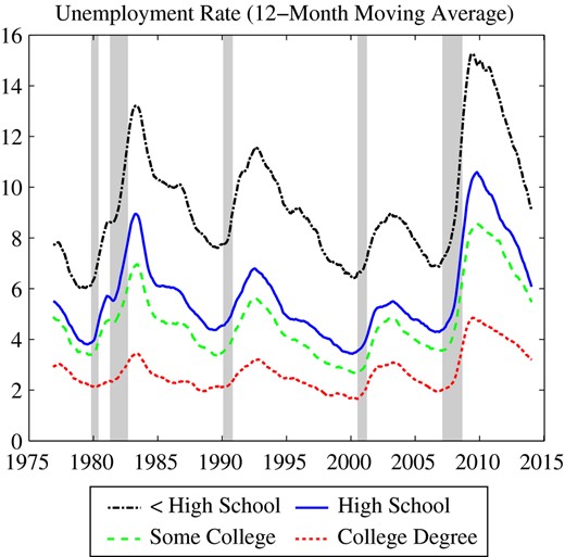
Unemployment Rate by Education (in %, 25+ years)
note. Colour figure can be viewed at wileyonlinelibrary.com
Theoretically, differences in unemployment across education groups can arise either because the more educated find jobs faster, because the less educated get fired more often, or due to a combination of the two factors. Empirically, different education groups face roughly the same unemployment outflow rate (loosely speaking, the job finding rate). What creates the remarkably divergent patterns in unemployment by education is the unemployment inflow rate (the job separation rate). Why is it, then, that more educated workers lose their jobs less frequently and experience lower turnover rates?
This article’s main hypothesis is that employment stability rises with education because more educated workers also receive more on‐the‐job training and thus accumulate more match‐specific human capital. As argued by Becker (1964), higher amounts of specific training should reduce incentives of firms and workers to separate.2 In order to explore the validity of this hypothesis, this article provides novel empirical evidence on unemployment dynamics by required job training. In particular, we construct unemployment rates, job finding rates and separation rates by specific vocational preparation as measured in the Dictionary of Occupational Titles (DOT). This evidence shows that highly educated workers are typically employed in occupations that require higher levels of specific vocational training. Moreover, workers in these occupations also experience substantially lower unemployment rates, which are due to lower separation rates. Even more strikingly, after we control for educational attainment, we find that higher levels of specific vocational training lead to substantially lower separation rates, but almost indistinguishable job finding rates.
Motivated by this empirical evidence, we develop a theoretical search and matching model with endogenous separations in the spirit of Mortensen and Pissarides (1994) and augment it with on‐the‐job training. In our model, all new hires lack some job‐specific skills, which they obtain through the process of initial on‐the‐job training. This training generates some match‐specific human capital, leading to higher job surplus and thus lower incentives to destroy a job. Consistent with empirical evidence, more educated workers engage in job activities that necessitate more initial on‐the‐job training and thus build a higher amount of specific human capital and experience lower separation rates than less educated workers.
We parameterise the model using micro evidence from the Employment Opportunity Pilot Project (EOPP) survey (the latter survey provides more detailed training measures than the DOT). In particular, our empirical measure of training for each education group is based on the duration of initial on‐the‐job training and the productivity gap between new hires and incumbent workers; both components rise considerably by education. The simulation results demonstrate that, given the observed differences in initial on‐the‐job training, the model is able to explain the empirical regularities across education groups on job finding, separation and unemployment rates, both in their first and second moments. This cross‐sectional quantitative success of the model is quite remarkable – especially when compared to the well‐documented difficulties of the canonical search and matching model to account for the main time‐series properties of aggregate labour market data (Shimer, 2005) – and thus represents the main contribution of this article.
Perhaps the most interesting aspect is the ability of the model to generate vast differences in the separation rate, whereas at the same time the job finding rate remains very similar across education groups. The result that on‐the‐job training leaves the job finding rate unaltered reflects two opposing forces. On the one hand, higher training costs lower the value of a new job, leading to less vacancy creation and a lower job finding rate. On the other hand, higher training costs reduce the probability of endogenously separating once the worker has been trained, implying a higher value of a new job and a higher job finding rate. The simulation results reveal that both effects cancel out; thus, an increase in training costs leaves the job finding rate virtually unaffected. This result is important because it cannot be obtained with standard models in the literature.
The model in this article can also be used to quantitatively evaluate several alternative explanations for differences in unemployment dynamics by education. In particular, the model nests the following alternative explanations that are based on differences in:
(i) job profitability (match surplus heterogeneity);
(ii) hiring costs;
(iii) frequency of idiosyncratic productivity shocks; and
(iv) dispersion of idiosyncratic productivity shocks.
Our article contributes to three strands of literature. First, it contributes to the theoretical literature of business‐cycle fluctuations that attempts to move beyond the representative agent framework. The aim of this literature is twofold: first, to test the plausibility of different theories by taking advantage of cross‐sectional data, and, second, to further our understanding of business‐cycle fluctuations by studying the heterogeneous effect of aggregate shocks on different demographic groups, which seems particularly relevant for fluctuations in the labour market. Relative to the existing contributions (Kydland, 1984; Gomme et al., 2005), we carry out our analysis within the equilibrium search and matching framework and find that the inability of this class of models to explain aggregate unemployment fluctuations at business‐cycle frequencies (Shimer, 2005) is not due to a failure of these models to account for fluctuations experienced by some particular education group, but instead this models’ failure pertains equally to all education groups. Moreover, this article shows that a tractable extension of the benchmark search and matching model delivers a framework that can account well for the cross‐sectional differences in unemployment fluctuations by education and can be thus fruitfully utilised for studying cross‐sectional labour market phenomena.
Second, our article contributes to the theoretical literature on search and matching models with worker heterogeneity. Contributions in this literature include Albrecht and Vroman (2002), Gautier (2002), Pries (2008), Dolado et al. (2009), Gonzalez and Shi (2010) and Krusell et al. (2010). However, in these papers, the worker’s exit to unemployment is assumed to be exogenous, hence they cannot be used to explain why the empirical unemployment inflow rate differs dramatically by education. Bils et al. (2012) allow for endogenous separations and heterogeneity in the rents from being employed; however, the latter assumption generates a substantial variation in the job finding rate and thus cannot be used to explain why the unemployment outflow rate empirically exhibits low variation by education. Relative to the existing literature, this article provides a search and matching model with endogenous separations and on‐the‐job training, which can generate substantial variability in job separation rates and at the same time small differences in job finding rates, which was a challenge for existing models.
Third, our article contributes to the empirical literature that studies cross‐sectional differences in unemployment dynamics by education. Using Panel Study of Income Dynamics (PSID) data, Mincer (1991) finds that the incidence of unemployment is far more important than the reduced duration of unemployment in creating the educational differentials in unemployment rates; he attributes this finding to higher amount of on‐the‐job training for more educated workers. Moreover, Elsby et al. (2010) obtain a similar finding of nearly identical outflow rates and different inflow rates across education groups in the Current Population Survey (CPS) data. Our article provides novel empirical evidence on unemployment dynamics by training requirements, where the latter are measured in the DOT. We find that workers in occupations with higher levels of training requirements experience substantially lower unemployment rates due to lower separation rates and this finding is present even after we control for educational attainment. In the article, we then use a combination of microdata and a theoretical model of equilibrium unemployment in order to discriminate quantitatively among several possible explanations for the observed empirical patterns.
Following this introduction, Section 1 provides empirical evidence on unemployment flows by education, on‐the‐job training by education and unemployment dynamics by training requirements. Section 2 outlines the model, which is then calibrated in Section 3. Section 4 contains the main simulation results of the model and a discussion of the mechanism driving the results. In Section 5 we quantitatively explore other possible explanations for differences in unemployment dynamics by education. Finally, Section 6 concludes with a discussion of possible avenues for further research.
1. Empirical Evidence
1.1. Unemployment Flows By Education
It is a well‐known and documented empirical fact that the unemployment rate differs by education (recall Figure 1). In the United States, the jobless rate of high school dropouts is almost four times greater than that of college graduates and this difference has been maintained since the data have been available. Moreover, the educational unemployment gap cannot be explained by standard demographic controls.3 Theoretically, a higher unemployment rate could be a result of a higher probability of becoming unemployed (a higher incidence of unemployment) or a lower probability of finding a job (higher duration of the unemployment spell). In order to distinguish between these possibilities, we follow the recent approach in the literature by calculating empirical unemployment inflows and outflows.4 As can be seen from Figure 2, outflow rates from unemployment for people 25 years of age and over are broadly similar across education groups, whereas inflow rates differ considerably, as already shown by Elsby et al. (2010).5 Moreover, these results are robust to the possible bias due to duration dependence and the inclusion of transitions in and out of the labour force (Cairó and Cajner, 2014).
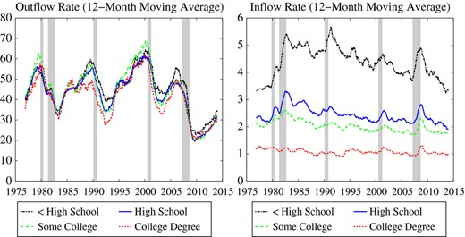
Unemployment Flows by Education (in %, 25+ years)
note. Colour figure can be viewed at wileyonlinelibrary.com
Table 1 provides standard deviations of the detrended data for the main labour market variables of interest.6 As shown in the Table, more educated workers enjoy not only lower risk of unemployment on average but also greater employment stability over the business cycle. The more educated experience also lower volatility of separation rates, whereas job finding rates exhibit broadly similar variation across education groups.
Labour Market Volatility By Education (In %, 25+ Years)
| Unemployment rate | Job finding rate | Separation rate | |
|---|---|---|---|
| Less than high school | 2.04 | 8.72 | 0.48 |
| High school | 1.40 | 8.01 | 0.27 |
| Some college | 1.09 | 9.25 | 0.20 |
| College degree | 0.59 | 9.14 | 0.17 |
| Unemployment rate | Job finding rate | Separation rate | |
|---|---|---|---|
| Less than high school | 2.04 | 8.72 | 0.48 |
| High school | 1.40 | 8.01 | 0.27 |
| Some college | 1.09 | 9.25 | 0.20 |
| College degree | 0.59 | 9.14 | 0.17 |
Note. Volatility is defined as the standard deviation of the data expressed in deviations from an HP trend with smoothing parameter .
Thus, in order to understand why the least educated workers have unemployment rates nearly four times greater and three times more volatile than the most educated workers, one has to identify economic mechanisms that create differences in the level and volatility of their inflow rates to unemployment.
1.2. On‐The‐Job Training and Education
Existing empirical studies of on‐the‐job training overwhelmingly suggest the presence of strong complementarities between education and training. The positive link between formal schooling and job training has been found in the following datasets:
(i) the CPS Supplement of January 1983, the National Longitudinal Surveys (NLS) of Young Men, Older Men and Mature Women, and the 1980 EOPP survey (Lillard and Tan, 1986);
(ii) the NLS of the High School Class of 1972 (Altonji and Spletzer, 1991);
(iii) PSID (Mincer, 1991); and
(iv) a dataset of a large manufacturing firm (Bartel, 1995).7
In what follows we provide some further evidence on training by education level from the 1982 EOPP survey, which will form the empirical basis for the parameterisation of our model. Table 2 summarises the main training variables of the survey with a breakdown by education.8
Measures of Training By Education
| Less than high school | High school | Some college | College degree | All individuals | |
|---|---|---|---|---|---|
| Incidence of initial training (%) | 94.0 | 94.5 | 97.0 | 95.1 | 95.0 |
| Time to become fully trained (weeks) | 10.2 | 12.0 | 15.9 | 18.2 | 13.4 |
| Productivity gap (%) | 32.5 | 36.2 | 45.3 | 48.1 | 39.1 |
Notes. The sample from the 1982 EOPP survey includes 1,053 individuals 25 years of age and older, for whom we have information on education. The distribution of training duration is truncated at its 95th percentile. All measures of training are mean averages and correspond to typical new hires.
The EOPP survey, which measures both formal and informal types of training, shows that almost all new hires (i.e. about 95%) receive some type of training during the first three months of their job, regardless of their level of education. However, there are considerable differences across education groups in terms of the duration of training received and the corresponding productivity gap, with the latter being defined as the percentage difference in productivity of an incumbent worker with two years of experience and a new hire. For example, a newly hired college graduate needs 18.2 weeks on average to become fully trained, which is nearly two times the time needed for a newly hired high school dropout. Moreover, the difference between the initial productivity and the productivity achieved by an incumbent worker increases with the education level as well, from one third to one half, indicating that more educated workers need to obtain a greater amount of job specific skills after being hired.9
The objective of this article is to study whether the observed differences in on‐the‐job training are able to explain the observed differences in unemployment rates across education groups quantitatively by affecting the job separation margin. In particular, the article’s main hypothesis claims that higher investments in training reduce incentives for job destruction. However, as argued already by Becker (1964) these incentives crucially depend on the portability of training across different jobs. As we argue below, there are strong reasons to believe that our empirical measure of on‐the‐job training can indeed be interpreted as being largely job‐specific and hence unportable across jobs.
First, the appropriate theoretical concept of specificity in our case is not whether a worker can potentially use his learned skills in another firm. What matters for our analysis is whether after going through an unemployment spell, a worker can still use his past training in a new job. To give an example, a construction worker might well be able to take advantage of his past training in another construction firm but, if after becoming unemployed he cannot find a new job in the construction sector and is thus forced to move to another sector, where he cannot use his past training, then his training should be viewed as specific. Industry and occupational mobility are not merely a theoretical curiosity but, as shown by Kambourov and Manovskii (2008), a notable feature of the US labour market, especially for workers that go through an unemployment spell. Similarly, by analysing the National Longitudinal Survey of Youth data, Lynch (1991) reaches the conclusion that on‐the‐job training in the United States appears to be unportable from employer to employer.
Second, the EOPP was explicitly designed to measure the initial training at the start of the job (as opposed to training in ongoing job relationships), which is more likely to be of job‐specific nature. Moreover, the EOPP also provides data on the productivity difference between the actual new hire during his first two weeks and the typical worker who has been in this job for two years. For the actual new hire the EOPP also reports months of relevant experience.10 Table 3 summarises the productivity differences between the actual new hire and the typical incumbent for three age groups and two levels of relevant working experience. Note that one would expect to observe in the data a rapidly disappearing productivity gap (between incumbents and new hires) with rising age of workers and months of relevant experience, if this measure of on‐the‐job training were capturing primarily general human capital.11 However, the results in Table 3 indicate that initial on‐the‐job training remains important also for older cohorts of workers and for workers with relevant experience. Crucially for our purposes, the relative differences across education groups remain present for older workers.12 Overall, this suggests that initial on‐the‐job training, at least as measured by the EOPP survey, contains primarily specific human capital.
Productivity Gap Between Incumbents and New Hires By Education
| Less than high school | High school | Some college | College degree | All individuals | |
|---|---|---|---|---|---|
| Productivity gap (mean, in %) | |||||
| 16 years and over | 32.2 | 35.4 | 37.9 | 43.9 | 36.4 |
| 25 years and over | 24.6 | 29.3 | 37.9 | 39.3 | 31.8 |
| 35 years and over | 20.2 | 29.3 | 31.7 | 38.6 | 29.6 |
| 25 years and over and at least | |||||
| 1 year of relevant experience | 22.7 | 24.5 | 34.4 | 41.7 | 28.8 |
| 5 years of relevant experience | 18.2 | 22.6 | 26.6 | 38.9 | 25.0 |
Notes. The productivity gap is calculated from the 1982 EOPP survey as the difference in productivity between the actual new hire and the typical incumbent worker. We restrict the sample to individuals for whom we have information on education.
1.3. Unemployment Dynamics by Training Requirements
In order to test the link between unemployment and training further, we provide here novel empirical evidence on unemployment dynamics by training requirements. The measure of training we use here is specific vocational preparation (SVP) as measured in the fourth edition of the DOT, provided by the US Department of Labor. The DOT defines specific vocational preparation as ‘the amount of lapsed time required by a typical worker to learn the techniques, acquire the information, and develop the facility needed for average performance in a specific job‐worker situation’. Following the methodology of Autor et al. (2003), we aggregate detailed occupations from DOT into three‐digit census occupation codes and then merge training data from these aggregated occupations with the CPS microdata to construct unemployment rates, job finding rates and separation rates by training requirements.
Figure 3 depicts unemployment dynamics by training requirements for all individuals 25 years of age and over (left panels) and for high school graduates 25 years and over (right panels). Given the strong complementarities between education and job training, it is not surprising to see that higher training requirements are associated with lower unemployment rates (top left panel). What is more striking is that even after we control for education, for example by focusing on high school graduates (top right panel), higher training levels remain to be related to more stable employment. Crucially, after we condition for educational attainment, higher levels of job training lead to empirically similar job finding rates (middle right panel), but much lower separation rates (bottom right panel).13 We view this novel empirical evidence, which shows that workers in occupations with higher specific vocational training experience substantially lower unemployment rates due to lower separation rates, as further support for the theoretical mechanism advocated in this article.
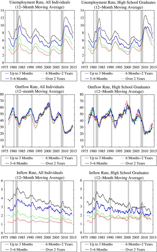
Unemployment Dynamics by Training Requirements (in %, 25+ years)
note. Colour figure can be viewed at wileyonlinelibrary.com
2. The Model
We proceed by constructing an equilibrium model of the labour market, which will be used to examine possible explanations for the empirical patterns of unemployment dynamics by education quantitatively. The model is an extension of the canonical search and matching model with endogenous separations (Mortensen and Pissarides, 1994). In our setting, workers initially lack some job‐specific skills, which they obtain during a period of on‐the‐job training. Consistent with the empirical evidence presented in the previous Section, more educated workers require a greater amount of on‐the‐job training for exogenous, technological reasons. The assumption of exogenous on‐the‐job training is made purposely, with the rationale being that initial on‐the‐job training is not something that a firm can freely decide whether to offer or not, since without this initial training workers cannot adequately perform all tasks of their job. Moreover, this assumption is also consistent with the particular empirical measure of job training used in this article, that is initial on‐the‐job training in the EOPP survey.
2.1. Environment
The discrete‐time model economy contains a finite number of segmented labour markets, indexed by , where h represents different levels of formal educational attainment. Workers in each of these markets possess a certain amount of formal human capital, denoted by , directly related to their education. Moreover, firms in each of these markets provide initial on‐the‐job training to their new hires, with the amount of training depending on worker’s education. The assumption of segmented labour markets is chosen because education is an easily observable and verifiable characteristic of workers, hence firms can direct their search toward desired education level for their new hires.14
Each segmented labour market features a continuum of measure one of risk‐neutral and infinitely‐lived workers. These workers maximise their expected discounted lifetime utility defined over consumption, , where β ∈ (0, 1) represents the discount factor. Workers can be either employed or unemployed. Employed workers earn wage , whereas unemployed workers have access to home production technology, which generates consumption units per time period. In general, also includes potential unemployment benefits, leisure, saved work‐related expenditures, and it is net of job‐searching costs. Importantly, it depends on worker’s education. We abstract from labour force participation decisions, therefore all unemployed workers are assumed to be searching for jobs.15
2.2. Labour Markets
2.3. Characterisation of Recursive Equilibrium
Note that the unemployed worker always starts as a trainee after finding a job, due to the initial lack of job‐specific skills. The assumption that on‐the‐job training is specific and thus lost upon separation is consistent with empirical evidence in subsection 1.2.
The model features a recursive equilibrium, with its solution being determined by 1234567891011. The solution of the model consists of equilibrium labour market tightness θ(H, A) and reservation productivity thresholds and . Next, the following proposition establishes an important neutrality result (see the online Appendix for the proof).
Under the assumptions and with c, b, H > the solution of the model is independent of H.
The usefulness of Proposition 1 will become clear in the following two Sections with calibration and numerical results of the model. In particular, the Proposition’s result enables a transparent comparison of the model results across different education groups h, with the only parameters affecting results being on‐the‐job training parameters. Notably, by using the Proposition we avoid changing the surpluses by magnifying the difference between the firm’s output and the value of being unemployed. We believe that the model’s implications when changing the value of being unemployed relative to output have been well explored in the recent literature.17 Indeed, by assuming that more educated workers enjoy higher match surplus (with being lower relative to output than in the case of less educated workers) it is well documented that the model would predict a decrease in the unemployment and the separation rate but at the same time it would also predict an increase in the job finding rate. The latter prediction strongly contradicts the empirical evidence across education groups, as documented in Section 1. Further discussion of these issues together with empirical evidence justifying the assumptions of proportionality in and is provided in the next Section.
3. Calibration
This Section provides details on the model calibration. First, we discuss the calibration of parameter values that are consistent with empirical evidence at the aggregate level. Second, we specify on‐the‐job training parameter values that are specific to each education group.
3.1. Parameter Values At the Aggregate Level
The model is simulated at monthly frequency. Table 4 summarises the parameter values at the aggregate level. The value of the discount factor is consistent with an annual interest rate of 4%. The efficiency parameter γ in the matching function targets a mean monthly job finding rate of 43.5%, consistent with the CPS microevidence for people 25 years and over as described in subsection 1.1. For the elasticity of the Cobb–Douglas matching function with respect to unemployment we draw from the evidence reported in Petrongolo and Pissarides (2001) and accordingly set α = 0.5. In the absence of any further microevidence, we follow most of the literature and put the workers’ bargaining power equal to η = 0.5. As we show in the online Appendix this guarantees efficiency of the equilibrium, consistent with the Hosios condition.
Parameter Values At the Aggregate Level
| Parameter | Interpretation | Value | Rationale |
|---|---|---|---|
| β | Discount factor | 0.9966 | Interest rate 4% p.a. |
| γ | Matching efficiency | 0.334 | Job finding rate 43.5% (CPS) |
| α | Matching function elasticity | 0.5 | Petrongolo and Pissarides (2001) |
| η | Worker’s bargaining power | 0.5 | Hosios condition |
| c | Vacancy posting cost | 0.11 | 1982 EOPP survey |
| b | Value of being unemployed | 0.71 | Hall and Milgrom (2008) |
| Standard deviation for log aggregate productivity | 0.0058 | Labour productivity (BLS) | |
| Autoregressive parameter for log aggregate productivity | 0.99 | Labour productivity (BLS) | |
| Mean log idiosyncratic productivity | −0.02 | Normalisation | |
| Standard deviation for log idiosyncratic productivity | 0.39 | Separation rate 2.2% (CPS) | |
| λ | Probability of changing idiosyncratic productivity | 0.3333 | Fujita and Ramey (2012) |
| δ | Exogenous separation rate | 0.007 | JOLTS data |
| ϕ | Probability of training upgrade | 0.3226 | 1982 EOPP survey |
| τ | Training costs | 0.196 | 1982 EOPP survey |
| H | Worker’s productivity | 1 | Normalisation |
For the parameterisation of the vacancy posting cost we take advantage of the EOPP data, which contain information on vacancy duration and hours spent during the recruitment process. In our sample, it took on average 17.8 days (or 0.59 month) to fill the vacancy, with 11.3 hours (or 6.5% of total working hours in a month) being spent during the whole recruitment process.18 Following the calculation procedure in Hall and Milgrom (2008), the expected recruitment cost in the model is equal to the product of the flow vacancy posting cost and the expected duration of the vacancy, c × (1/q). Hence, we have on a monthly basis c × 0.59 = 0.065 (we implicitly assume that recruiters have the same productivity as hired workers, where the average productivity of the latter is normalised to 1). This gives us the flow vacancy posting cost c = 0.11 or about 11% of average worker’s productivity, essentially the same as in Hagedorn and Manovskii (2008) and very similar to other parameter values used in the literature.
The flow value of non‐market activities b in general consists of several elements, including:
(i) unemployment insurance benefits;
(ii) home production and self‐employment;
(iii) value of leisure and disutility of work;
(iv) expenditures saved by not working; and
(v) it is net of job‐searching costs.
Parameters for the Markov chain governing the aggregate productivity process are calibrated to match the cyclical properties of the quarterly US labour productivity between 1976 and 2014.19 After taking logs and deviations from an HP trend with smoothing parameter , the standard deviation of quarterly labour productivity equals 0.017 and its quarterly autocorrelation is 0.89. We apply the Rouwenhorst (1995) method for finite state Markov‐chain approximations of AR(1) processes, which has been found to generate accurate approximations to highly persistent processes (Kopecky and Suen, 2010).
In choosing the Markov chain for the idiosyncratic productivity process, we follow the standard assumption in the literature by assuming that idiosyncratic shocks are independent draws from a lognormal distribution with parameters and . As in Fujita and Ramey (2012), these draws occur on average every quarter (λ = 1/3), governing the persistence of the Markov chain. In order to determine the parameters of the lognormal distribution and the exogenous separation rate we match the empirical evidence on separation rates. The CPS microevidence for people 25 years of age and over gives us a mean monthly inflow rate to unemployment of 2.2%. Following again Fujita and Ramey (2012), we assume that two thirds of all separations are endogenous (1.5%). Note that this is consistent with the recent Job Openings and Labor Turnover Survey (JOLTS) data, available from December 2000 onwards, which yield the mean monthly layoff rate of about 1.5%; the layoffs in JOLTS data correspond to separations initiated by the employer, hence we can interpret these as endogenous separations. Accordingly, we set the exogenous monthly separation rate to δ = 0.007 and adjust in order that the simulated data generate mean monthly inflow rates to unemployment of 2.2%. The parameter is set to −0.02, which normalises the average worker’s productivity to 1.
We select parameters regarding on‐the‐job training from the 1982 EOPP survey as summarised in Table 2. To calibrate the duration of on‐the‐job training, we consider the time to become fully trained in months. In particular, for the aggregate economy we parameterise the average duration of on‐the‐job training to 3.10 months (13.4 weeks times 12/52), which yields the value for ϕ equal to 1/3.10. To calibrate the extent of on‐the‐job training we use the average productivity gap between a typical new hire and a typical fully trained worker. In reality, we would expect that workers obtain job‐specific skills in a gradual way, i.e. shrinking the productivity gap due to lack of skills proportionally with the time spent on the job. Our parameterisation of training costs for the aggregate economy, τ = 0.196, implies that trainees are on average 19.6% less productive than skilled workers. This is consistent with an average initial gap of 39.1%, which is then proportionally diminishing over time. Finally, the worker’s human capital parameter H is normalised to one.
3.2. Parameter Values Specific to Education Groups
Next we turn to parameterising the model across education groups. We keep fixed all the parameter values at the aggregate level as reported in Table 4, with the only exception being the training parameters (ϕ and τ). In particular, we assume that and , making applicable the neutrality result of Proposition 1, according to which the parameterisation for H is irrelevant and we normalise it to 1. We argue below that this is not only desirable from the model comparison viewpoint, as we can completely isolate the effects of on‐the‐job training, but it is also a reasonable assumption. Note also that a neutrality result similar to Proposition 1 would obtain if we were to assume a standard utility function in macroeconomic literature, featuring disutility of labour and offsetting income and substitution effects (Blanchard and Galí, 2010).
Regarding the parameterisation of , recall that this parameter should capture several elements, including unemployment insurance benefits, home production, disutility of work, expenditures saved by not working and job‐searching costs. Intuitively, higher educational attainment could lead to higher through all of the mentioned elements. More educated workers typically earn higher salaries and are hence also entitled to higher unemployment insurance benefits due to the statutory link between past wages and unemployment benefits (albeit the latter are usually capped at some level). Higher educational attainment presumably not only increases market productivity but also home production, which incorporates the possibility of becoming self‐employed. Jobs requiring more education could be more stressful, leading to higher disutility of work, and might require higher work‐related expenditures (e.g. commuting, meals, clothing). Finally, more educated workers might be able to take advantage of more efficient job‐searching methods, lowering their job‐searching costs. Overall, this supports our benchmark assumption that .20
The proportionality assumption on the flow vacancy posting cost would follow directly if we were to assume that hiring is a labour intensive activity as in Shimer (2009). Moreover, the textbook matching model also assumes proportionality of hiring costs to productivity (Pissarides, 2000). Nevertheless, in Cairó and Cajner (2014) we perform the sensitivity analysis of the quantitative results with respect to different specification of vacancy posting cost and show that the results are robust to different parameterisations of the flow vacancy posting cost.
For the parameters regarding on‐the‐job training by education group, we follow the same calibration strategy as in the aggregate case but, of course, using the empirical counterparts as reported in Table 2. Moreover, we report all on‐the‐job training parameter values for different education groups in tables with simulation results.
4. Simulation Results
The main results of the article are presented in this Section. First, we report simulation results for the aggregate economy. Second, the model is solved and simulated for each education group. This exercise is done by changing the parameters and related to on‐the‐job training for each education group, while keeping the rest of parameters fixed at the aggregate level. Finally, we discuss the main mechanism of the model, by exploring how simulation results depend on each training parameter. Details of the computational strategy are available in the online Appendix.
4.1. Simulation Results at the Aggregate Level
We begin by simulating the model, parameterised at the average aggregate level for duration of training and training costs (1/ϕ = 3.10 and τ = 0.196). Table 5 reports simulation results for the aggregate economy together with the actual data moments for the US during 1976–2014.
Labour Market Variables: Data Versus Model
| u | f | s | |
|---|---|---|---|
| Panel (a): US data, 1976–2014 | |||
| Mean | 5.07 | 43.46 | 2.19 |
| Volatility | 1.13 | 8.06 | 0.20 |
| Panel (b): Model simulation results | |||
| Mean | 4.88 | 43.48 | 2.19 |
| (0.60) | (2.33) | (0.16) | |
| Volatility | 0.47 | 1.86 | 0.13 |
| (0.16) | (0.37) | (0.04) | |
Notes. u refers to unemployment rate, f to job finding rate, and s to separation rate. Statistics for the model in panel (b) are means (in %) across 1,000 simulations, standard deviations across simulations are reported in parentheses.
The simulation results show that the model performs reasonably well at the aggregate level. It essentially hits the empirical means of the job finding rate and the separation rate by construction of the exercise. It underpredicts the empirical volatilities somewhat but this result is well known in the search and matching literature and it should not be surprising given that in this model productivity shocks are the only cause of labour market fluctuations (as shown by Mortensen and Nagypál, 2007, the empirical correlation between labour productivity and labour market tightness is 0.396, thus, substantially below the model’s correlation of close to 1).
4.2. Unemployment Dynamics across Education Groups
Next, Table 6 shows the simulation results when we vary the training parameters across education groups (keeping the rest of the parameter values at the aggregate value). The model is able to explain the differences in unemployment rates across education groups that we observe in the data. In particular, the ratio of unemployment rates of the least educated group to the most educated group is 3.4 in the data and 3.3 in the model. Moreover, the model accounts for the observable differences in separation rates across groups, while keeping similar job finding rates. The ratio of separation rates of the least educated group to the most educated group is 4.0 in the data and 3.5 in the model. In general, the greater the degree of on‐the‐job training (longer training periods and higher productivity gaps), the lower is the separation rate and the lower is the unemployment rate. In sum, the observed variation in training received across education groups can explain most of the observed differences in separation rates and unemployment rates, while keeping similar job finding rates.
Education, Training, and Unemployment Dynamics: Means
| Data | Parameters | Model | ||||||
|---|---|---|---|---|---|---|---|---|
| u | f | s | u | f | s | |||
| Less than high school | 9.29 | 45.23 | 4.37 | 2.35 | 0.163 | 7.64 | 43.28 | 3.53 |
| (0.77) | (2.15) | (0.20) | ||||||
| High school | 5.72 | 43.18 | 2.44 | 2.78 | 0.181 | 6.10 | 43.21 | 2.76 |
| (0.68) | (2.17) | (0.18) | ||||||
| Some college | 4.70 | 44.34 | 2.03 | 3.67 | 0.227 | 3.04 | 43.58 | 1.34 |
| (0.38) | (2.33) | (0.10) | ||||||
| College degree | 2.71 | 41.05 | 1.08 | 4.19 | 0.240 | 2.30 | 43.70 | 1.01 |
| (0.25) | (2.34) | (0.06) | ||||||
Note. Statistics for the model are means (in %) across 1,000 simulations, with standard deviations across simulations reported in parentheses.
Table 7 reports the simulation results for volatilities. As already mentioned, the model suffers somewhat from the unemployment volatility puzzle. Nevertheless, the model replicates the relative differences in volatilities across education groups well. In the data, the volatility of the unemployment rate for high school dropouts is 3.4 times higher than the corresponding volatility for college graduates, whereas the same ratio in the model stands at 3.2. Something similar is true for volatilities of separation rates (the ratio is 2.8 in the data and 3.9 in the model). The model can also account for the observed similar values of volatilities in job finding rates across education groups.
Education, Training and Unemployment Dynamics: Volatilities
| Data | Parameters | Model | ||||||
|---|---|---|---|---|---|---|---|---|
| u | f | s | u | f | s | |||
| Less than high school | 2.04 | 8.72 | 0.48 | 2.35 | 0.163 | 0.64 | 1.79 | 0.18 |
| (0.17) | (0.35) | (0.04) | ||||||
| High school | 1.40 | 8.01 | 0.27 | 2.78 | 0.181 | 0.56 | 1.82 | 0.16 |
| (0.16) | (0.36) | (0.04) | ||||||
| Some college | 1.09 | 9.25 | 0.20 | 3.67 | 0.227 | 0.30 | 1.89 | 0.08 |
| (0.10) | (0.37) | (0.03) | ||||||
| College degree | 0.59 | 9.14 | 0.17 | 4.19 | 0.240 | 0.20 | 1.90 | 0.05 |
| (0.07) | (0.37) | (0.02) | ||||||
Notes. Volatility is defined as the standard deviation of the data expressed in deviations from an HP trend with smoothing parameter . Statistics for the model are means (in %) across 1,000 simulations, with standard deviations across simulations reported in parentheses.
In order to provide another view of the model’s results, we conduct the following experiment. Using the model’s original solution for the aggregate economy and the actual data on the aggregate unemployment rate we back out the implied realisations of the aggregate productivity innovations.21 Then, we feed this implied aggregate productivity series to the model’s solution for each education group. The simulated unemployment rate series for each group are shown in Figure 4, together with the actual unemployment rates. Again, the model replicates the data well.
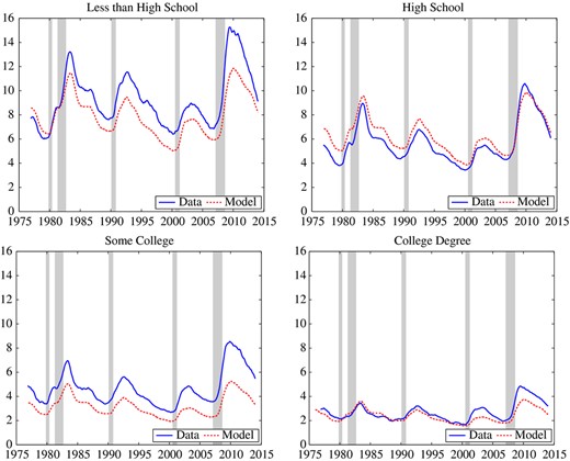
Unemployment Rates by Education (in %): Model Versus Data
Notes. We plot 12‐month moving averages. The simulated unemployment rates are generated by solving and simulating the model for each education group, using the implied realisations of the aggregate productivity innovations as explained in the text. Colour figure can be viewed at wileyonlinelibrary.com
4.3. Discussion of the Model’s Mechanism
In order to highlight the mechanism at work in our model, we analyse separately the effects of training duration (left panel of Figure 5) and productivity gap of new hires (right panel of Figure 5); in both cases, we keep the rest of the parameters constant at the aggregate level. We find that both components of training quantitatively play almost equally important roles for our results. In particular, we observe a decrease in the mean of the unemployment rate as we increase the degree of on‐the‐job training (longer training periods and higher productivity gaps). This decrease in the unemployment rate is completely driven by the decrease in the separation rate, given that the job finding rate remains roughly constant as we vary the degree of on‐the‐job training.
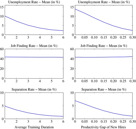
The Role of On‐the‐job Training Parameters
Note. The left (right) panel studies the role of the average training duration (productivity gap of new hires), keeping the rest of parameters constant at the aggregate level. Colour figure can be viewed at wileyonlinelibrary.com
Let us consider first why the job finding rate virtually does not move with the average duration of on‐the‐job training. One would expect that an increase in the average duration of on‐the‐job training reduces the value of a new job, since the worker spends more time being less productive. Consequently, firms’ incentives to post vacancies should decrease, leading to a decrease in the job finding rate. However, an increase in the average duration of on‐the‐job training also reduces the probability of separating endogenously once the worker becomes fully trained. This second effect increases the value of a new job and, hence, incentives for vacancy posting go up. It turns out that these two effects cancel out and the job finding rate hence remains almost unaffected. The same reasoning holds for the productivity gap of new hires, which measures the extent of on‐the‐job training. Again, we have two effects at work, which cancel each other out; a higher extent of on‐the‐job training by itself decreases the value of a new job but, at the same time, the latter increases through lower endogenous separations of fully trained workers.
In order to understand why separation rates decrease with the degree of on‐the‐job training, Figure 6 shows the reservation productivity thresholds for trainees and fully trained workers for different degrees of on‐the‐job training. As we can see, investments in match‐specific human capital do not significantly affect the incentives of trainees to separate but they clearly do so for fully trained workers. The intuition for this result is that fully trained workers know that upon a job loss they will have again to undergo a period of on‐the‐job training with a lower wage. Hence, reservation productivity levels drop for fully trained workers as we increase the degree of on‐the‐job training, implying a lower rate of endogenous separations.
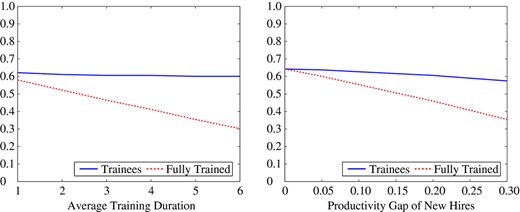
The Effects of On‐the‐job Training on Reservation Productivity
Note. The left (right) panel plots reservation productivity for trainees and fully trained workers for different training durations (productivity gaps of new hires), keeping the rest of parameters constant at the aggregate level. Colour figure can be viewed at wileyonlinelibrary.com
The assumption that on‐the‐job training is specific is important for our results. If we instead assumed that training is general, the worker’s outside option would be permanently higher after being trained, which would in turn dampen the effect of training on the reservation threshold. More precisely, the worker’s productivity would be permanently higher and thus firms would post more vacancies for trained workers, which would in turn raise the job finding rate for trained workers and, as argued above, would make them more likely to get separated in comparison with the case when training is specific. Nevertheless, workers who received more general training would still have lower separation rates than workers with less general training, since their productivity would be higher.22 Additionally, our model could be extended to allow for heterogeneity in the loss of training upon becoming unemployed, similarly as in Ljungqvist and Sargent (1998, 2007). Such an extension would be valuable for analysing issues like long‐term unemployment (where the loss of human capital is likely to be larger) and sectoral worker mobility (where the loss of human capital is likely to be larger when an unemployed worker finds a job in a different sector).23
4.4. Wage Implications
One additional labour market aspect in which individuals differ by educational attainment is wages. Given Proposition 1, our model can easily match empirical differences in wage levels by education. We confirmed this theoretical result by calibrating H in line with empirical wage differentials as measured in hourly EOPP wages; as expected, the simulated unemployment dynamics remained the same as reported in Tables 6 and 7 but the model now also matched empirical wage differences across groups. Moreover, given the well‐known result by Hall (2005) that any wage in the bargaining set is consistent with equilibrium in search and matching models, our model is well suited to match not only differential wage levels but also differential wage dynamics by education. On the other hand, this general property of search and matching models can also be viewed as a weakness and more research is needed in order to provide a more informative link between wage implications of these models and empirical evidence on wage dynamics.
5. Evaluating Other Potential Explanations
This Section evaluates the plausibility of other potential explanations for differential unemployment dynamics by education. In particular, our model can encompass the following alternative hypotheses that are based on differences in:
(i) size of match surplus;
(ii) hiring costs;
(iii) frequency of idiosyncratic productivity shocks; and
(iv) dispersion of idiosyncratic productivity shocks.
Other Potential Explanations
| u | f | s | |
|---|---|---|---|
| Panel (a): US data, 1976–2014 | |||
| Less than high school | 9.29 | 45.23 | 4.37 |
| High school | 5.72 | 43.18 | 2.44 |
| Some college | 4.70 | 44.34 | 2.03 |
| College degree | 2.71 | 41.05 | 1.08 |
| Panel (b): Size of match surplus | |||
| 12.02 | 31.83 | 4.20 | |
| 7.29 | 38.25 | 2.93 | |
| 4.52 | 44.59 | 2.08 | |
| 2.98 | 50.40 | 1.53 | |
| Panel (c): Hiring costs | |||
| 10.77 | 53.06 | 6.33 | |
| 5.55 | 44.56 | 2.57 | |
| 3.25 | 39.63 | 1.31 | |
| 2.45 | 35.69 | 0.89 | |
| Panel (d): Idiosyncratic shocks – frequency | |||
| 17.48 | 31.21 | 6.57 | |
| 11.37 | 37.85 | 4.81 | |
| 4.90 | 43.41 | 2.20 | |
| 1.41 | 49.95 | 0.71 | |
| Panel (e): Idiosyncratic shocks – dispersion | |||
| 11.72 | 38.84 | 5.09 | |
| 8.31 | 40.85 | 3.65 | |
| 5.49 | 42.85 | 2.44 | |
| 3.32 | 45.11 | 1.52 | |
Notes. Statistics for the model are means (in %) across 1,000 simulations. Subscript 1 denotes less than high school, 2 high school, 3 some college, and 4 college degree.
5.1. Differences in the Size of Match Surplus
One possibility why more educated workers enjoy higher employment stability might be related to higher profitability of their jobs. In the terminology of search and matching framework, more educated workers might be employed in jobs yielding a higher match surplus. The latter crucially depends on the worker’s outside option, which is in turn governed by the flow value of being unemployed. In our main simulation results as reported in Section 4, we ruled out this possibility by assuming proportionality between the flow value of being unemployed and labour market productivity across education groups.
Here we relax the proportionality assumption and instead assume that the size of match surplus is increasing with education: , , , . The simulation results, reported in panel (b) of Table 8, indicate that the unemployment rate decreases with education under this alternative parameterisation, as in the data. However, the model now counterfactually predicts higher job finding rates for more educated workers. Intuitively, since jobs with more educated workers yield higher surplus, firms are willing to post more vacancies in this segment of the labour market, leading in turn to higher labour market tightness and job finding rates.
As discussed in subsection 3.2, the assumption that match surplus rises with education also lacks empirical support in the US data. Interestingly, Gomes (2012) reports evidence that in the UK both the differences in job finding and separation rates contribute roughly equally toward generating differences in unemployment rates by education. OECD data also show that the average of net replacement rates over 60 months of unemployment is roughly twice as high in the UK as in the US.24 To the extent that this difference in net replacement rates reflects more generous welfare policies in the UK, which would in turn invalidate our baseline assumption of proportionality between market and non‐market returns, differences in the size of match surplus might play a role for explaining unemployment dynamics by education in countries with more generous welfare policies.
5.2. Differences in Hiring Costs
Another possible explanation for differences in unemployment dynamics by education might be related to hiring costs. One could imagine that hiring costs are greater for highly skilled individuals and anecdotal evidence about head hunters in some top‐skill occupations would be consistent with such a story. In our main simulation results in Section 4, we already assumed that flow vacancy posting costs are growing proportionally with productivity. However, it might be that this assumption understates the true differences in hiring costs by education.
In what follows, we assume the following values for vacancy posting costs, which are expressed in terms of output: , , , . Hence, hiring somebody with a college degree is now four times costlier than hiring a high school dropout in terms of their output.25 The simulation results, reported in panel (c) of Table 8, reveal that under the assumed differences in hiring costs the model replicates the unemployment rates by education. However, the model now predicts sharply decreasing job finding rates with education, which is in contrast with the empirical evidence. What is the economic mechanism behind these simulation results? Because it is costlier to hire college graduates, firms will post fewer vacancies in this labour market segment. As a consequence, their job finding rate drops. Highly educated workers that are currently employed know that upon a job loss they will face a lower job finding rate, hence they are less likely to get separated than less educated workers. The less educated workers are instead facing high job finding rates, hence they are more willing to leave their employer in the case of low idiosyncratic productivity shock.
5.3. Differences in Frequency of Idiosyncratic Productivity Shocks
Individuals with different educational attainment might work in different industries and occupations (e.g. blue‐collar and white‐collar workers). Therefore, it might be that differences in unemployment dynamics by education are due to industry and/or occupation specific factors.26 But then the natural question is in what sense industries and occupations differ. It is quite likely that they differ in terms of initial on‐the‐job training requirements and this would be consistent with our main story, according to which differences in training lead to differences in unemployment. However, it might also be the case that industries and occupations are subject to heterogeneous dynamics of idiosyncratic shocks. For example, industries and occupations with predominantly low educated workers might be subject to more frequent shocks.
The simulation results reported in panel (d) of Table 8 illustrate what happens when we vary the Poisson arrival rate of idiosyncratic productivity shocks from every six months (λ = 1/6) to every two months (λ = 1/2). It turns out that the faster the arrival rate of idiosyncratic productivity shocks, the lower will be the separation rate. The intuition behind this result is straightforward: if new shocks arrive often, then it is better to stay in the match even in the case of a very low idiosyncratic productivity shock, since you avoid the unemployment spell.27 But these results are then not consistent with the notion that it should be the industries and occupations with low educated workers (blue‐collar jobs) that are facing more frequent shocks. Additionally, the model fails to generate similar job‐finding rates.
5.4. Differences in Dispersion of Idiosyncratic Productivity Shocks
Still another possibility, related to the story from the previous subsection, is that the dispersion of idiosyncratic productivity shocks varies across industries and occupations (or more generally, across jobs with different proportions of workers by education). This possibility is explored in panel (e) of Table 8. The results show that higher dispersion of idiosyncratic productivity shocks generates more separations and leads to higher unemployment. But this would then imply that low educated workers should exhibit higher wage dispersion than high educated workers, which is at odds with the empirical evidence. In particular, the evidence provided in Chen (2008) for the United States using data from the National Longitudinal Survey of Youth shows that college graduates have higher variance of wages than high school graduates, even after controlling for individual fixed effects. Furthermore and similar as before, this model specification also cannot generate similar job finding rates in the presence of different unemployment rates.
5.5. Other Alternative Explanations
The model presented in this article clearly cannot be used to examine all alternative explanations for differences in unemployment dynamics by education quantitatively. Here we briefly comment on some alternatives not nested by our model and compare them to the available empirical evidence.
First, it is theoretically possible that more educated workers make job‐to‐job transitions more frequently and are consequently better matched and more insulated from job separation risk than low educated workers. However, following the methodology from Fallick and Fleischman (2004), we calculated job‐to‐job transitions by education for individuals 25 years and over from the micro CPS data and it turns out that high school graduates have essentially the same job‐to‐job transition rate as college graduates (for both groups the average monthly job‐to‐job transition rate between 1994 and 2014 was 1.9%).
Second, individuals could differ in their preferences for job security and these preferences could be correlated with the education level.28 However, the evidence presented in subsection 1.3 shows that even after controlling for education, higher levels of job training lead to much lower separation rates (and similar job finding rates). Additionally, if preferences for job security were correlated with education, this would presumably lead to differences in job‐to‐job transitions by education as well but, as argued above, such differences are not present in the data. Furthermore, empirical work by Shaw (1996) finds that risk aversion actually falls significantly with education, in contrast with the proposed hypothesis examined here.
Third, risk aversion also could potentially play a role in explaining unemployment dynamics by education in a setting with incomplete markets and asset accumulation. However, in such a theoretical setting individuals with lower assets would be less willing to separate from a job (Bils et al., 2011), while in the data low educated individuals have lower assets than high educated and at the same time experience higher separation rates.29 Thus, differences in assets are unlikely to explain the observed patterns in unemployment dynamics by education.
Fourth, minimum wages, which are more likely to bind for less educated workers, could potentially explain their higher unemployment rates. Nevertheless, the empirical research following Card and Krueger (1994) finds conflicting evidence on the effect of minimum wages on employment. If anything, the employment effects of minimum wages appear to be empirically modest (Dube et al., 2010).
Finally, Sengul (2015) presents a theoretical model in which differences in separation rates by education are driven by differential recruitment selection technology and by differential speed of learning about match quality. We view these mechanisms as complementary to the training channel advocated in this article and more empirical evidence on the selection technology and the speed of learning about match quality by education would be valuable to understand their quantitative implications better.
6. Conclusions
In this article, we build a theoretical search and matching model with endogenous separations and initial on‐the‐job training. We use the model in order to explain differential unemployment properties across education groups. The model is parameterised by taking advantage of detailed micro evidence from the EOPP survey on the duration of on‐the‐job training and the productivity gap between new hires and incumbent workers across four education groups. In particular, the applied parameter values reflect strong complementarities between educational attainment and on‐the‐job training. The simulation results reveal that the model almost perfectly captures the empirical regularities across education groups on job finding rates, separation rates and unemployment rates, both in their first and second moments. The on‐the‐job training explanation for the differential unemployment dynamics by education is also validated by the novel empirical evidence provided in this article, which shows that workers in occupations with higher training requirements experience much lower separation rates, but similar job finding rates than those in occupations with low training requirements.
The analysis of this article views training requirements as a technological constraint, inherent to the nature of the job. We believe that such a view is appropriate for the initial on‐the‐job training, for which we also have exact empirical measures that are used in the paper for the parameterisation of the model. However, in reality, firms also provide training to their workers in ongoing job relationships. To investigate such cases it would be worthwhile to endogenise the training decisions and examine interactions between training provision and job separations. We leave these extensions for future research.
Footnotes
Except where noted otherwise, the data in this article are constructed from the monthly Current Population Survey (CPS) microdata. The sample period is from 1976:01 to 2014:12.
For more details, see Cairó and Cajner (2014).
See, for example, Elsby et al. (2009) and Shimer (2012). Details of the procedure to construct flows, which are based on the unemployment duration data, can be found in the online Appendix. Note that in this article, we use interchangeably expressions ‘inflow rate’ and ‘separation rate’, as well as ‘outflow rate’ and ‘job finding rate’.
There is an older literature, which is not based on empirical unemployment flows, that also attributes unemployment differences by education to the incidence of unemployment (Ashenfelter and Ham, 1979; Nickell, 1979; Mincer, 1991). Indeed, evidence on the effect of education on unemployment duration in that literature is mixed, with some studies finding a negative effect (Nickell, 1979; Mincer, 1991), some negligible effect (Ashenfelter and Ham, 1979), and some positive effect (Moffitt, 1985; Meyer, 1990).
To detrend, we use an HP filter with a smoothing parameter of . Some papers in the literature express variables in natural logarithms when calculating volatilities. In our case, however, this leads to a distorting effect due to different means across education groups. For further discussion and volatility measures of the data expressed in natural logarithms, see Cairó and Cajner (2014).
The survey question for training duration was: ‘How many weeks does it take a new employee hired for this position to become fully trained and qualified if he or she has no previous experience in this job, but has had the necessary school‐provided training?’. Since the distribution of training duration is highly skewed to the right, we eliminate outliers by truncating distribution at its 95th percentile, which corresponds to the training duration of two years. In order to compute the productivity gap we combine the survey question on productivity of a ‘typical worker who has been in this job for two years’ and the survey question on productivity of a ‘typical worker during his/her first two weeks of employment’.
The EOPP survey also reports numbers of training hours in the first three months, which show very similar differences by education: high school dropouts receive 87 training hours, high school graduates 133 hours, people with some college 142 hours, and college graduates 170 hours.
The exact survey question was ‘How many months of experience in jobs that had some application to the position did (NAME) have before (he/she) started working for your company?’.
This evidence could be also consistent with training that represents updating of skills to keep up with the latest techniques. Nevertheless, under this interpretation training shares the property of being effectively lost (outdated) over time (especially during unemployment), similar to the features of specific training.
Consistent with our hypothesis, also the differential in the separation rates remains present as people age (see Table B1 in the online Appendix B). We leave the analysis of interactions between on‐the‐job training and unemployment flows over the life cycle for future research.
This result is true for all four education groups as shown in Table B2 in the online Appendix.
In a somewhat related setting with direct search, Mortensen and Pissarides (1999) show that even if one allows for the possibility of overqualification, whereby workers can apply for jobs that require lower formal education than their own, workers optimally self‐select themselves into appropriate educational sub‐markets, yielding a perfectly segmented equilibrium. For the contrasting case with random search, see for example Pries (2008).
As argued in subsection 1.1, flows in and out of the labour force are not crucial for explaining the educational unemployment gap.
Related modelling approaches are adopted in Kambourov and Manovskii (2009) and Silva and Toledo (2009). Silva and Toledo (2009) model on‐the‐job training without workers’ heterogeneity in order to examine the issue of aggregate volatilities in the search and matching model. Kambourov and Manovskii (2009) abstract from business‐cycle fluctuations and use their occupation‐specific human capital model with experienced and inexperienced workers to investigate occupational mobility and wage inequality.
The survey questions were ‘Approximately how many days were between the time you started looking for someone to fill the opening and the time new hire started to work?’ and ‘While hiring for this position, what was the total number of man hours spent by your company personnel recruiting, screening, and interviewing all applicants?’. We restrict the sample to individuals 25 years of age and older, for whom we have information on education. Because of positive skewness, the vacancy duration and the hours spent distributions are truncated at their 99th percentiles, which correspond to six months and 100 hours, respectively.
Following Shimer (2005), labour productivity is the seasonally adjusted real output per job in the nonfarm business sector (series PRS85006163 provided by the Bureau of Labor Statistics).
While more detailed empirical evidence on this issue is scarce, Aguiar and Hurst (2005) report that during unemployment food expenditure and food consumption fall by similar proportion for low and high educated. Moreover, the recent paper by Chodorow‐Reich and Karabarbounis (2016) finds that across education groups the flow value of the opportunity cost of employment is proportional to the after‐tax marginal product of employment, supporting our benchmark assumption. Results from robustness checks on our benchmark assumption are provided in Cairó and Cajner (2014).
Of course, given that the model suffers somewhat from the unemployment volatility puzzle, the backed‐out productivity realisations are more volatile than those observed in the data.
Another technicality in the case with general training is about who pays for this type of training. Becker (1964) argued that in the case of competitive labour markets, only workers will be willing to pay for general training. However, in a setting with search frictions, the worker and the firm can share the costs of general training (Acemoglu and Pischke, 1999). See also Wasmer (2006) who allows for endogenous investments in either specific or general human capital and studies how these investments depend on labour market institutions.
Relatedly, Laureys (2014) studies the externality effect of human capital depreciation on job creation.
See http://www.oecd.org/els/benefits‐and‐wages‐statistics.htm.
Acknowledging differences in their productivity, this implies that in absolute terms hiring costs are more than six times higher for the most educated group relative to the least educated group.
Results from estimated regression equations in Cairó and Cajner (2014) indicate that this might indeed be part of the story.
Note that non‐linearities are present here: after some point, lower frequency of idiosyncratic productivity shocks leads to slowly declining separation rates.
Relatedly, Jarosch (2014) investigates a case where jobs differ in terms of job security and workers are homogeneous.
For empirical evidence on net worth by education from the Survey of Consumer Finances, see Bricker et al. (2014).
References
Author notes
The analysis and conclusions set forth are those of the authors and do not indicate concurrence by other members of the research staff or the Board of Governors. We are especially grateful to Jordi Galí and Thijs van Rens for their guidance, advice and encouragement. We thank Morten Ravn (the editor), three anonymous referees, Regis Barnichon, Fabio Canova, Vasco Carvalho, Nir Jaimovich, Christian Merkl, Pascal Michaillat, Claudio Michelacci, Stacey Tevlin, Antonella Trigari, Eran Yashiv and numerous seminar audiences for valuable comments and suggestions. We also thank Vera Brenčič for help with the EOPP data. This research was conducted when both authors were graduate students at Universitat Pompeu Fabra and they gratefully acknowledge financial support during that period from the Spanish Ministry of Science and Innovation, the Government of Catalonia and the European Social Fund.
