


Abstract
We present the first results of the eXtreme UV Environments (XUE) James Webb Space Telescope (JWST) program, which focuses on the characterization of planet-forming disks in massive star-forming regions. These regions are likely representative of the environment in which most planetary systems formed. Understanding the impact of environment on planet formation is critical in order to gain insights into the diversity of the observed exoplanet populations. XUE targets 15 disks in three areas of NGC 6357, which hosts numerous massive OB stars, including some of the most massive stars in our Galaxy. Thanks to JWST, we can, for the first time, study the effect of external irradiation on the inner (<10 au), terrestrial-planet-forming regions of protoplanetary disks. In this study, we report on the detection of abundant water, CO, 12CO2, HCN, and C2H2 in the inner few au of XUE 1, a highly irradiated disk in NGC 6357. In addition, small, partially crystalline silicate dust is present at the disk surface. The derived column densities, the oxygen-dominated gas-phase chemistry, and the presence of silicate dust are surprisingly similar to those found in inner disks located in nearby, relatively isolated low-mass star-forming regions. Our findings imply that the inner regions of highly irradiated disks can retain similar physical and chemical conditions to disks in low-mass star-forming regions, thus broadening the range of environments with similar conditions for inner disk rocky planet formation to the most extreme star-forming regions in our Galaxy.
Export citation and abstract BibTeX RIS

Original content from this work may be used under the terms of the Creative Commons Attribution 4.0 licence. Any further distribution of this work must maintain attribution to the author(s) and the title of the work, journal citation and DOI.
1. Introduction
The formation history of exoplanetary systems is constrained by comparing the demographics of the observed exoplanet population to the properties of planet-forming disks. Until the arrival of JWST, disks for which we were able to determine the composition and their physical structure (e.g., mass, radius) were all located in nearby (<500 pc) regions. However, observations (Stolte et al. 2010; Guarcello et al. 2016; Eisner et al. 2018; van Terwisga et al. 2019) and theory (Fatuzzo & Adams 2008; Winter et al. 2020) converge on the idea that well-studied disks (in regions such as Taurus and Lupus) are not typical, as most (>50%) stars and planetary systems form in massive star-forming regions (e.g., Krumholz et al. 2019), where they are exposed to intense UV radiation from nearby OB stars (Winter & Haworth 2022).
External photoevaporation by far-UV (FUV) photons (Winter et al. 2018) is expected to dominate over stellar encounters (Bate 2018) in most environments (Scally & Clarke 2001; Guarcello et al. 2016). External FUV fluxes ≳103 G0 can drive significant mass-loss rates from protoplanetary disks (PPDs). For instance, in the core of the Orion Nebula Cluster (ONC), at FUV fluxes of ≳5 × 10⁴ G0, mass-loss rates up to ∼10−6 M⊙ yr−1 are possible (Johnstone et al. 1998; Henney & O'Dell 1999; Adams et al. 2004; Facchini et al. 2016; Haworth et al. 2018). Due to these high mass-loss rates, the mass and dissipation timescale of the gaseous disk are reduced (Adams et al. 2004; Concha-Ramírez et al. 2019; Winter et al. 2020), resulting in rapid outer disk dispersal. This inhibits the growth and inward drift of dust particles from the outer disk (Sellek et al. 2020; Qiao et al. 2023) and the rate of pebble accretion needed for rapid growth from planetesimals to protoplanets. Rapid loss of gas and dust may curtail the growth of gas giants, resulting in entirely different planetary architectures.
Atacama Large Millimeter/submillimeter Array (ALMA) studies show that the cold dust reservoir in the outer disks near massive stars in Orion is depleted by photoevaporation (Mann et al. 2014; Ansdell et al. 2017; van Terwisga et al. 2019, 2020; van Terwisga & Hacar 2023). Some inner disk studies of a large sample of young massive star clusters, combining X-ray (Chandra) and infrared (Spitzer) data, have found correlations between disk lifetimes and UV flux, although this may depend on the mass or age of the region (Roccatagliata et al. 2011; Fang et al. 2012; Richert et al. 2015; Guarcello et al. 2016; Richert et al. 2018).
Several studies of disks around nearby solar-type stars with Spitzer report on the detection of rotational and rovibrational emission of molecules such as water, CO, OH, 12CO2, HCN, and C2H2 (Carr & Najita 2008; Pontoppidan et al. 2010; Salyk et al. 2011; Najita et al. 2013; Pascucci et al. 2013). These molecules trace warm gas and are typically found to be confined to the inner 5–10 au of PPDs (e.g., Glassgold et al. 2009; Najita et al. 2011; Woitke et al. 2018). Thanks to the increase of more than two orders of magnitude in sensitivity for JWST compared to Spitzer, we are able to extend these observations to larger distances (≥2 kpc). This allows us for the first time to study the physical properties and chemical composition of PPDs in extreme radiation regions.
With an age of 1–1.6 Myr (Getman et al. 2014) and located at a distance of ≃1.77 kpc (Kuhn et al. 2019, based on Gaia DR2 data), NGC 6357 is one of the youngest and closest massive star formation complexes, containing one of the most massive stars in our Galaxy (Pis24-1,O4III(f+)+O3.5If*; Walborn 2003) and more than 20 other O stars across the field. NGC 6357 has the great advantage that it allows us to probe different radiation environments in each of its three subclusters (Pismis 24, G353.1+0.6, and G353.2+0.7; Churchwell et al. 2007; Fang et al. 2012; Getman et al. 2014), which share the same age and distance but differ significantly in their FUV environment irradiating the PPDs (Russeil et al. 2010; Ramírez-Tannus et al. 2020). We reassess the distance to Pismis 24 using Gaia DR3 (Gaia Collaboration 2023) and find a distance of 1690 pc (see Appendix B).
The eXtreme UV Environments (XUE) program aims at characterizing the physical properties and chemical composition of 15 PPDs in NGC 6357 with the Medium Resolution Spectrometer (MRS) of the Mid-InfraRed Instrument (MIRI). In this paper we focus on the PPD XUE 1 (17:24:40.098, −34:12:25.55). XUE 1 is located in the subregion Pis24 near the O-star binary Pis24-1. We infer an age of ≈0.7 Myr for this source, which corresponds to the median age of the stars in its vicinity (see Table 6 of Getman et al. 2022), based on the PARSEC 1.2S age scale. Due to its location near several massive stars in NGC 6357, we expect XUE 1 to have been constantly exposed to a high radiation field throughout its life (∼105 G0; A. Winter et al. 2023, in preparation). This unlike irradiated disks in the ONC, where a single O star (θ1 C) dominates the UV flux, and therefore PPDs migrate in and out of the proplyd regime (∼5 × 10⁴ G0) in short periods of time (∼0.1 Myr).
In this paper we explore the impact of externally driven photoevaporation on PPDs located in an extreme FUV environment using MIRI MRS spectroscopy. We report on the chemical inventory of the inner few au of XUE 1. By means of LTE and non-LTE slab models, we determine the temperature, column density, and emitting area of each of the molecules and compare our findings with those for isolated, nearby disks around stars of similar mass. In Section 2 we present the observational strategy and the data reduction. Section 3 reports on the results, and in Section 4 we discuss and conclude this work.
2. Observations
In this section we present the observations of XUE 1. In Section 2.1 we show the photometric observations of our target, and in Section 2.2 we describe the MIRI MRS Observations.
2.1. Near-infrared Photometry
XUE 1 is part of a triple system (see Appendix A) where the third star (B) is at a distance of 1 5 (∼2600 au) from a binary system (A1+A2) whose components are ≈02 (∼300 au) apart. Based on the MIRI imaging, we conclude that A1 is the star with the PPD giving rise to the observed MIRI spectrum (see Appendix A).
We derive the masses of XUE 1 A1 and XUE 1 A2 from their extinction-corrected z-band magnitudes (zA1 ≃ 17.9 mag and zA2 ≃ 18.9 mag). We assume that both components are subject to the same extinction AV ∼ 8.7 mag as derived for the unresolved object A using UKIRT photometry (Broos et al. 2013; King et al. 2013). The z band is not much affected by the presence of accretion/disks, and assuming a reddening law of Az /AV = 0.505 (Rieke & Lebofsky 1985), the comparison with the PARSEC 1.2S models (Chen et al. 2014; Tang et al. 2014; Chen et al. 2015) for the 0.7 Myr isochrone gives the masses MA1 ≈ 1.1 M⊙ and MA2 ≈ 0.6 M⊙ for a distance of 1690 pc.
2.2. JWST-MIRI MRS Spectra
XUE 1 was observed on 2022 August 3 as part of the XUE project in Cycle 1 (GO-1759; Ramirez-Tannus et al. 2021) with the MIRI MRS (Rieke et al. 2015; Wells et al. 2015; Wright et al. 2015). All three wavelength settings (SHORT, MEDIUM, and LONG) are used for the observations. A four-point dither optimized for a point source was performed in the negative direction. The observations are obtained in the FASTR1 readout mode with 40 groups per integration and 2 integrations per dither position. This results in a total exposure time of 900 s per wavelength setting and 2700 s in total. No dedicated background observations were taken for this observation. The background in the observation is dominated by the emission of the surrounding H ii region and photodissociation region and spatially highly variable.
We reduced the data using the JWST Pipeline version 1.9.4, with context 1046 of the Calibration Reference Data System (CRDS; Bushouse et al. 2023). The Detector1 part of the pipeline was run without modifications. In Spec2 we implemented a custom background subtraction. After the WCS assignment, we performed a background subtraction by removing the two nodding positions from each other. This minimizes the effect of the variable background with respect to taking a dedicated background observation. We then run the standard steps in Spec2, including the residual fringe correction. In Spec3, we skipped the outlier rejection step, as it causes artifacts in the extracted spectrum owing to the undersampling of the point-spread function. The final cubes are combined using the drizzle algorithm.
Both components A (A1+A2) and B are visible in the MRS data cubes, but the two components in source A are not resolved. To identify the disk-bearing source, we used archival Hubble Space Telescope (HST)/Advanced Camera for Surveys (ACS) imaging from the Hubble Legacy Archive and the simultaneous MIRI F560W imaging corresponding to our program (see Appendix A). We measured the position of source A in the datacube and ran the extract1d step with the position of the source as input. We extracted the source with a modified aperture 2 times smaller than the default value, linearly increasing from 03 at 5 μm to 128 at 22 μm. We use the aperture corrections corresponding to this extraction aperture. The full 4.9–22 μm spectrum of XUE 1 is shown in Figure 1.

Figure 1. MIRI MRS spectrum of XUE 1. The most prominent dust features are labeled. The insets show the P-branch transitions of the CO rovibrational fundamental band, the water emission around 7 μm, and the 13–15 μm region featuring C2H2, HCN, and 12CO2.
Download figure:
Standard image High-resolution image3. Results
The spectrum of XUE 1 presented in Figure 1 shows a rising continuum from warm dust in the disk surface layers with amorphous silicate emission at 10 and 18 μm, as well as forsterite features at 16.3 and 20 μm. The shape and strength of the dust features are typical for passive disks heated by stellar photons. In addition to the dust features, the MIRI spectrum displays a wealth of molecular emission from H2O, CO, HCN, C2H2, and 12CO2. In this section we first present the temperature derivation of the CO fundamental via the rotation diagram. Then, we describe the results of the modeling procedure with slab models. The detailed spectral analysis leading to this section is described in Appendix C.
3.1. CO
We detect the P-branch CO fundamental emission between 4.9 and 5.35 μm with upper J levels between 24 and 46 for the v = 1 − 0 transitions and between 19 and 41 for the v = 2 − 1 transitions. Using the rotational diagram method (Goldsmith & Langer 1999), we estimate the excitation temperature and column density of the CO molecule. We fit the unblended lines with Gaussian profiles to find their flux (see Table 2 in Appendix. C.1.1 for the measured fluxes). We then calculate their specific intensity by assuming that the emission originates from a disk annulus with a radius of 0.5 au (see below) and a distance of 1690 pc. The rotation diagrams in Figure 2 are consistent with straight lines, suggesting LTE and optically thin conditions. We derive excitation temperatures of Tex = 2883 ± 276 K for the v = 1−0 bands and of Tex = 2606 ± 568 K for the v = 2−1 bands. A different choice of emitting area and/or distance would only affect the absolute values for the column densities but does not change the temperature estimate or the relative column density of v = 1−0 with respect to v = 2−1.

Figure 2. Rotation diagrams for the v = 1−0 (circles), v = 2−1 (triangles) bands. The dashed and dotted lines show linear fits to each vibrational level.
Download figure:
Standard image High-resolution imageThe fact that we can perform linear fits for each vibrational level indicates that the rotational level populations within each vibrational level are in LTE. However, the measured column densities of the v = 2−1 bands are lower than those of v = 1−0, indicating that collision partner densities are not high enough to significantly populate the v = 2−1 level, requiring non-LTE level populations (see also Appendix C).
We fit radex non-LTE slab models (van der Tak et al. 2007) to the v = 1 − 0 and v = 2 − 1 bands simultaneously, including blended lines, following the methodology described in Tabone et al. (2023) (see Appendix C.1.2 for more details). The best-fitting non-LTE model for CO is shown in the top panel of Figure 3, and the best-fitting parameters are listed in Table 1. It has a temperature of 2300 K, which is consistent with the results from the rotation diagrams. The best-fitting column density is N = 3 × 1017 cm−2, and the emitting radius is R = 0.44 au. The density of collisional partners (see Appendix C) of the best-fitting model is n<H> = 6 × 1012 cm−3, which is close to the critical density for v = 1 − 0 (Thi et al. 2013). This indicates that collisions populate the rotational levels within the v = 0 according to LTE, but the densities are too low to bring the vibrational temperature to the gas temperature. The temperature is well constrained to values between 2000 and 2800 K, and N is well constrained to values between 1016 and 1018 cm−2 (see χ2 map, in Appendix D). However, it has been shown that including the low-energy lines, not present in the MIRI spectrum, could lead to higher column densities and lower temperatures (e.g., Banzatti et al. 2022). Near-IR (∼4.2–5 μm) observations are needed to better constrain the CO fundamental's physical parameters. In order to fit the CO lines to the slab models, we need a lower resolution than that of the MRS at 5 μm (Argyriou et al. 2023). The CO lines are spectrally resolved with a deconvolved FWHM of 51 km s−1. Assuming that the emission originates in a disk annulus and Keplerian rotation, we can calculate the characteristic radius. We adopt a mass of 1 M⊙ and, as the inclination is not known, assume a value of 60° for XUE 1. This results in a characteristic radius of 0.25 ± 0.09 au, which is in agreement with the best-fitting slab model. Assuming an edge-on disk would lead to a radius of 0.34 au, while an inclination of 30° would result in a 0.09 au radius.

Figure 3. Continuum-subtracted MIRI spectrum of XUE 1 (black) with the best-fit slab models. Molecules are shown with colors, and the purple shaded area shows the total model spectrum. Top: region between 4.9 and 5.35 μm including CO (brown) and H2O (blue). Bottom: region between 13 and 16 μm including H2O (blue), C2H2 (green), HCN (orange), and 12CO2 (red).
Download figure:
Standard image High-resolution imageTable 1. Best-fit Model Parameters for the Studied Molecules
| Species | N | T | R |

| 〈n〉H | N0.5 au | T0.5 au | |
|---|---|---|---|---|---|---|---|---|
| (cm−2) | (K) | (au) | (mol.) | (cm−3) | (K) | |||
| H2O [7 μm] | 2.2 × 10¹⁸ | 975 | 0.13 | 2.6 × 1043 | ⋯ | 6.8 × 10¹⁶ | 1150 | |
| H2O [15 μm] | 6.8 × 10¹⁹ | 550 | 0.46 | 1.0 × 1046 | ⋯ | 2.2 × 10¹⁹ | 575 | |
| HCN | 2.2 × 10¹⁷ | 575 | 0.57 | 5.0 × 1043 | ⋯ | 4.6 × 10¹⁶ | 675 | |
| C2H2 | 2.2 × 10¹⁸ | 475 | 0.23 | 8.2 × 1043 | ⋯ | 3.2 × 10¹⁷ | 550 | |
| CO2 | 2.2 × 10¹⁴ | 450 | 5.30 | 4.3 × 1042 | ⋯ | 3.2 × 10¹⁶ | 450 | |
| CO | 3.0 × 10¹⁷ | 2300 | 0.44 | 4.1 ×1043 | 6.0 × 10¹² |
Note. Columns (2), (3), (4), (5), and (6) show the disk properties obtained when leaving the radius as a free parameter. Columns (7), and (8) show the N, and T for a radius of 0.5 au.
Download table as: ASCIITypeset image
3.2. Spectral Region between 6 and 17 μm
We fit the spectra of water around 7 μm and in the 13–17 μm region with LTE slab models (Tabone et al. 2023; see Appendix C.2 for details). The bottom panel of Figure 3 shows the best-fit model to the spectral region between 13 and 16.3 μm, and the best-fit model parameters for each molecule are listed in Table 1. The χ2 maps resulting from the fitting procedure for each molecule are shown in Appendix D. From these maps it is possible to read the typical uncertainties on the best-fit parameters; the red, orange, and yellow lines show the 1σ, 2σ, and 3σ levels, respectively. In addition to the three free parameters (T, N, and R), we also list the total number of molecules ( ), which is well constrained for optically thin emission.
3.2.1. H2O
Many H2O emission lines are present in the spectrum of XUE 1, both in the region around 7 μm, corresponding to the bending mode, and in the region around 15 μm, corresponding to rotationally excited lines. For the fitting, we include emission of both ortho- and para-H2O assuming a typical ratio ortho/para = 3 (e.g., Herczeg et al. 2012; Mottram et al. 2014; Herpin et al. 2016; Putaud et al. 2019). The region from 6 to 8 μm is best represented by an LTE slab model with T = 975 K, N = 2.2 × 1018 cm−2, and an emitting area given by R = 0.13 au, whereas the 13–17 μm region is best reproduced by a model with T = 550 K, N = 6.8 × 1019 cm−2, and an emitting area given by R = 0.46 au. For the hotter H2O we can exclude temperatures <300 K, but the upper limit on the temperature is poorly constrained. For the cooler H2O component the temperature is better constrained to values between ∼450 and ∼700 K. It has been pointed out in the literature that the shorter wavelengths probe H2O at higher temperatures, while the longer wavelengths probe the colder regions (Blevins et al. 2016; Banzatti et al. 2023; Gasman et al. 2023). For XUE 1, although the best-fitting values agree with this behavior, when taking into account the confidence intervals, the temperature cascade does not seem to be as extreme, similarly to the case in PDS 70 (Perotti et al. 2023).
3.2.2. 12CO2
We detect the 12CO2 Q-branch at 14.9 μm. The best-fitting model for 12CO2 has a temperature of 450 K, a column density of 2.2 × 1014 cm−2, and an emitting area given by R = 5.3 au. Nevertheless, the column density is in the optically thin regime, so N and R are degenerate. The temperature is well constrained to values between 300 and 650 K. We do not find evidence for the 12CO2 hot bands at 13.9 and 14.2 μm or for the presence of CO2 isotopologues as found by Grant et al. (2023) around the low-mass T Tauri star GW Lup. This supports our findings that CO2 is likely optically thin.
3.2.3. C2H2 and HCN
We detect the Q-branches of C2H2 and HCN around 13.7 and 14 μm, respectively, including the HCN hot band at 14.3 μm. For HCN the temperature is well constrained for a range between ∼550 and ∼650 K. For C2H2 the best-fitting models have temperatures between ∼300 and ∼800 K. We find column densities of 2.2 × 1017 cm−2 and 2.2 × 1018 cm−2 for HCN and C2H2, respectively. For C2H2 the best-fit model is in the optically thick regime, but models with higher temperatures and in the optically thin regime are not possible to exclude. From the best-fitting models we find emitting areas given by radii of R = 0.57 and 0.23 au. After subtracting all the best-fitting models to the observed spectrum, we do not find evidence for OH emission.
As 12CO2 and possibly C2H2 are in the optically thin regime, and therefore we cannot constrain R and N independently, we also calculate the best-fit parameters for an assumed radius of 0.5 au, based on radiative transfer models (Greenwood et al. 2019). The results of the latter are listed in the last three columns of Table 1.
4. Discussion and Conclusions
In this paper we present the first JWST-MIRI spectrum of an extremely irradiated PPD located in a 1 Myr old massive star-forming cluster. We detect H2O, CO, 12CO2, HCN, and C2H2 in its inner disk, as well as crystalline silicates.
4.1. Comparison to PPDs in Low-mass Star-forming Regions
We compare our measurements with Spitzer and newly obtained JWST observations of PPDs that are not strongly irradiated, i.e., in low-mass star-forming regions. Figure 4 shows the line luminosity of H2O, measured from the 17 μm lines, against the HCN/H2O, C2H2/H2O, CO/H2O, and 12CO2/H2O of XUE 1 in comparison with a sample of T Tauri stars located in nearby (<200 pc), young (1–3 Myr) star-forming regions from Banzatti et al. (2020, 2022) and the newly obtained JWST observations of isolated PPDs (Grant et al. 2023; Kóspál et al. 2023; Perotti et al. 2023). We find that the H2O luminosity and the 12CO2/H2O ratio are at the high end of the distribution. However, The HCN/H2O, C2H2/H2O, and CO/H2O ratios are higher than found in the T Tauri sample.
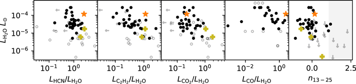
Figure 4. Comparison between the gas line luminosities and spectral index n13–25 of XUE 1 and the Spitzer sample studied by Banzatti et al. (2020) and the CO emission from Banzatti et al. (2022) (black circles). The y-axis shows the 17 μm H2O luminosity. From left to right the x-axis shows the ratio of HCN, C2H2, CO2, and CO to H2O luminosities. The x-axis of the rightmost panel shows the spectral index n13–25, where the shaded region shows the location of disks with large gaps and/or cavities. The measurements for the JWST spectrum of XUE 1 are shown with the orange stars. The upper limits from Banzatti et al. (2020) and Banzatti et al. (2022) are indicated with gray arrows, and the open circles show the sources with upper limits in both the numerator and denominator. The yellow plus signs show the location of the MIRI spectra published to date: GW Lup (Grant et al. 2023), EX Lup (Kóspál et al. 2023), and PDS 70 (Perotti et al. 2023).
Download figure:
Standard image High-resolution imageHigh line luminosities of molecular species are a signpost of a high-energy input into the disk, which can be intrinsic, i.e., due to a high stellar luminosity and/or a high gas accretion rate, or extrinsic, i.e., a strong external irradiation field, or a combination of these effects. Since the line luminosities of XUE 1 are in the range of those observed in nonirradiated disks (see Appendix E; but note the high C2H2 and HCN line luminosities; see below), disk irradiation is not needed to explain our observations.
Perotti et al. (2023) compare the H2O luminosity of a sample of disks from Banzatti et al. (2020, 2022) to the continuum spectral index n13–30, which is a measure of the dust depletion of the inner disk. We follow this approach, but we calculate the n13–25 from the Spitzer spectra from the Spexodisks database (Pontoppidan et al. 2010; Salyk et al. 2011; Banzatti et al. 2020) to allow direct comparison to our MIRI data. The right panel of Figure 4 shows that XUE 1 does not have a dust-depleted inner disk, which implies that the inner disk dust and gas content of XUE 1 is comparable to that of the average T Tauri disks in nearby low-mass star-forming regions.
In summary, we find no substantial evidence for an externally irradiated disk surface in XUE 1. This is surprising because models of disk spectra for continuous, irradiated disks show much stronger line enhancements than detected for XUE 1 (Antonellini et al. 2015). These strong line enhancements are the result of the entire disk surface being warm enough to contribute to the line emission. In the following we discuss two scenarios that can explain our observations, i.e., the disk is shielded from UV irradiation, or the disk is truncated.
4.2. Is XUE 1 Shielded from FUV Radiation?
A scenario in which XUE 1 is shielded from the UV radiation from the massive stars could explain why its spectral properties in the MIRI spectral range resemble those of nearby disks. The physical and chemical properties of the innermost parts of the disks traced by MIRI are dominated by the radiation from the central star. Therefore, if XUE 1 is shielded from the radiation, given the mass of the central star, there would be no reason to expect the MIRI MRS spectrum to be different from those of nearby regions. In the top panel of Figure 5 we show the extinction AK reported by Ramírez-Tannus et al. (2020) for a sample of stars in Pis24 including the extinction measured for XUE 1 in this work. The extinction toward XUE 1 does not seem higher than that of the neighboring stars. This is consistent with the lack of a significant dust cloud between XUE 1 and the O-type stars in the Herschel maps. However, the resolution of Herschel is not high enough to detect small-scale molecular features.

Figure 5. Top: extinction AK for a sample of stars in Pis24, shown in colors. The position of XUE 1 in this diagram is indicated with a star. The O stars from the bottom panel are indicated with magenta borders. Bottom: radiation field toward XUE 1. The lines show the 2D distance from the massive stars to XUE 1 (indicated with the black star), and the colors of the circles show their temperature. The FUV radiation felt by XUE 1 from each massive star is shown by the color and width of the lines.
Download figure:
Standard image High-resolution imageThe bottom panel of Figure 5 shows the projected distribution of massive stars (Teff ≥ 24,000 K) in Pis24 with respect to the position of XUE 1. The external FUV radiation felt by XUE 1 assuming a 2D projected distance is represented by the colors and width of the lines. The stars contributing the most to the FUV radiation are all located toward the left side of the plot. Given this asymmetric FUV radiation field, it is not possible to discard the presence of a coherent dust structure, like a filament, shielding XUE 1 from most of the external radiation.
Nevertheless, Getman et al. (2014) show that heavily embedded objects within clouds, such as XUE 1 (AV ≳ 10 mag), may undergo an environmental transformation due to cloud dispersal. These objects can become less absorbed (AV ∼ 5 mag) and thus be significantly influenced by the radiation emitted by nearby massive stars, on timescales of less than 0.5 Myr. Therefore, it is still possible that XUE 1 has been exposed to the UV radiation at some point during its evolution. It is also possible that XUE 1 and the massive stars are not exactly at the same distance. If that were the case, the FUV field felt by XUE 1 could be substantially lower than reported in Figure 5.
4.3. Is XUE 1's Disk Truncated?
Disk truncation would result in a change of the SED. Given the wavelength coverage of the MIRI MRS spectrum and the lack of longer-wavelength data, disks as small as a few au would all show a similar spectrum in the MIRI data, i.e., poorly constraining the outer disk radius. The line emission provides much stronger constraints on the disk outer radius. Antonellini et al. (2015) predict the mid-infrared emission of externally irradiated disks to be much stronger than in isolated disks. This is because of an increase of the line-emitting area. If XUE 1's disk were truncated, it would not be possible to form a hot layer of gas extending beyond the inner disk, and therefore the emitting area would be similar to that observed in nearby disks, which is dominated by the radiation from the central star and by accretion heating. Therefore, a truncation of XUE 1's disk could explain the fact that we do not see extraordinarily strong emission lines.
The observed HCN and C2H2 line luminosities of XUE 1 are higher than in the Banzatti sample, while this is not the case for 12CO2. We note that this is consistent with disk irradiation because in nonirradiated disks the C2H2 and HCN emission is more concentrated in the innermost disk, while 12CO2 has a larger emitting area. In an irradiated disk C2H2 and HCN will therefore be relatively more enhanced. However, we note that other effects, such as a higher inner disk C/O ratio (perhaps caused by a lower inward pebble flux), may also result in high C2H2 and HCN line luminosities.
Disk truncation may also be traced by the presence or absence of polycyclic aromatic hydrocarbon (PAHs). For PAHs to emit in their infrared vibrational resonances, they need to be exposed to a UV radiation field. T Tauri stars in low-mass star-forming regions only rarely show PAH emission (Geers et al. 2006). This is most likely due to a lack of a strong enough stellar UV radiation field. Indeed, In the hotter Herbig Ae/Be stars PAHs are much more frequently detected, particularly in sources with a large dust disk gap and/or inner disk dust depletion (Acke et al. 2010). The PAH emission in Herbig stars is dominated by the outer disk surface layers (e.g., Lagage et al. 2006; Yoffe et al. 2023) and traces the spatial distribution of gas. If the disk of XUE 1 is exposed to a radiation field G0 as high as indicated in the color bar of Figure 5, we expect the full gas disk surface to contribute to the PAH emission, because such radiation fields are similar to or exceed those provided by the central stars of disks surrounding Herbig stars. However, the background-subtracted spectrum of XUE 1 (Figure 1) does not show any evidence for PAH emission. The central star is probably too cool to produce sufficient UV photons. Assuming a similar abundance of PAHs in the disk of XUE 1 to that in disks surrounding Herbig stars, this suggests that any gaseous disk surrounding XUE 1 cannot be spatially very extended, unless the disk is shielded from UV radiation.
With the data at hand, it is possible to fully discard neither the extinction nor the disk truncation scenario. Nevertheless, given the evidence presented, we have a slight preference for the truncation scenario. Dedicated ALMA observations are needed to prove or disprove the hypothesis that XUE 1's disk is truncated. Additionally, we are performing a parameter study using the radiation thermochemical disk model ProDiMo (Woitke et al. 2009; Kamp et al. 2017), in which we study the effect of disk truncation and PAH abundance on the spectra of irradiated PPDs. With this study we will be able to better understand the MIRI MRS observations (S. Hernández et al. 2023, in preparation).
4.4. Consequences for Planetary System Formation
With this first observation of water and other molecules in the inner, terrestrial-planet-forming regions of a disk in one of the most extreme environments in our Galaxy, we show that conditions for (terrestrial) planet formation, routinely found in disks in low-mass star-forming regions, can also occur in massive star-forming regions. The fact that dust grain growth happens fastest in the inner disk (e.g., Birnstiel et al. 2012) and that there have been substructures detected in disks that could be caused by planets in systems at 0.5 Myr old (Sheehan & Eisner 2018; Segura-Cox et al. 2020) leaves the possibility that planet formation has already happened or has gone a long way at the age of XUE 1 (∼1 Myr). Therefore, the fact that XUE 1's disk might be truncated does not necessarily prohibit planet formation.
However, it is reasonable to expect different masses and orbital periods for the XUE 1's planets, compared to those that formed in lower UV environments. For example, if planets form by pebble accretion, then the young planets would be fed by a stream of pebbles from the outer disk. If the outer disk is dissipated, the supply of material that helps the planets grow is reduced (see, e.g., Qiao et al. 2023). Indeed, outer disk truncation due to UV radiation is well documented by ALMA observations (Ansdell et al. 2017; van Terwisga et al. 2019, 2020; van Terwisga & Hacar 2023), and our observations could be the first evidence based on MIRI observations that the outer disk radius in such an extreme environment has been truncated.
XUE 1 shows that the conditions for terrestrial planet formation can also happen in extreme environments. Nevertheless, the remaining observations from the XUE program are crucial to establish the frequency with which this occurs.
Acknowledgments
We thank the referee for constructive comments that helped improve the manuscript. M.C.R.-T. acknowledges support by the German Aerospace Center (DLR) and the Federal Ministry for Economic Affairs and Energy (BMWi) through program 50OR2314 "Physics and Chemistry of Planet-forming disks in extreme environments." A.B. acknowledges support from the Swedish National Space Agency (2022-00154). The research of C.G. and T.P. was supported by the Excellence Cluster ORIGINS, which is funded by the Deutsche Forschungsgemeinschaft (DFG, German Research Foundation) under Germany's Excellence Strategy—EXC-2094—390783311. T.J.H. acknowledges funding from a Royal Society Dorothy Hodgkin Fellowship and UKRI guaranteed funding grant (EP/Y024710/1). I.K. acknowledges support from grant TOP-1 614.001.751 from the Dutch Research Council (NWO) and funding from H2020-MSCA-ITN-2019, grant No. 860470 (CHAMELEON). G.P. gratefully acknowledges support from the Max Planck Society. V.R. acknowledges the support of the Italian National Institute of Astrophysics (INAF) through the INAF GTO grant "ERIS & SHARK GTO data exploitation." B.T. has received funding under the Horizon 2020 innovation framework program and Marie Sklodowska-Curie grant agreement No. 945298. The research of B.T. is also supported by the Programme National "Physique et Chimie du Milieu Interstellaire" (PCMI) of CNRS/INSU with INC/INP co-funded by CEA and CNES. A.J.W. has received support from the European Research Council (ERC) under the European Union's Horizon 2020 research and innovation program (PROTOPLANETS, grant agreement No. 101002188).
This work is based (in part) on observations made with the NASA/ESA/CSA James Webb Space Telescope. The data were obtained from the Mikulski Archive for Space Telescopes at the Space Telescope Science Institute, which is operated by the Association of Universities for Research in Astronomy, Inc., under NASA contract NAS 5-03127 for JWST. These observations are associated with program No. 1759, and the specific observations analyzed can be accessed via https://doi.org/10.17909/6nwv-6f56.
Facility: JWST (MIRI MRS) - James Webb Space Telescope.
Software: Astropy (Astropy Collaboration et al. 2013, 2018, 2022), NumPy (Harris et al. 2020), Matplotlib (Hunter 2007).
Appendix A: Optical/Near-infrared Counterpart of XUE 1
The original target of the MIRI observation was 2MASS J17244012–3412263 (J = 14.77, H = 12.34, K = 11.54). Inspection of the MIRI data revealed that there are actually two mid-infrared sources near this position, with an angular separation of about 15. The multiple nature of the source was confirmed by inspection of near-infrared images from the "VISTA VVV: ZYJHKs Catalogue in the Via Lactea, Release 3," where the northern component (A) has the source number vvv J172440.11−341225.39 (J = 15.07, H = 12.99, K = 12.80). The UKIRT magnitudes for this source are J = 14.93, H = 13.53, K = 12.59 (Broos et al. 2013; King et al. 2013). The southern component (B) has the source number vvv J172440.14−341226.70 (J = 15.14, K = 11.78). The mid-infrared source XUE 1 coincides very well with component A.
However, our inspection of the available optical HST/ACS archive images showed that the northern component A is again resolved into two point-like components (denoted as A1 and A2), with an angular separation of just about 02.
The left panel of Figure 6 shows the HST ACS F850LP image of XUE 1. The J2000 coordinates of the three components, as measured in this HST image, are (α, δ) = (17:24:40.100, −34:12:25.36) for A1, (17:24:40.098, −34:12:25.55) for A2, and (17:24:40.138, −34:12:26.84) for B. Component A1 coincides very well with the Gaia DR3 object 5976051168205228416, which has magnitudes G = 19.99, GBP = 21.66, and GRP = 18.43; unfortunately, the listed parallax of ϖ = (−0.66 ± 0.69) mas does not provide useful distance information.
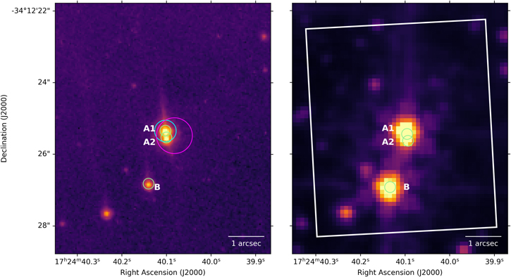
Figure 6. Left: HST/ACS F850LP band image of the target position for XUE 1. The three point-like objects are marked by green circles with radii of 01. The cyan circle on A1 marks the position of the Gaia DR3 source 5976051168205228416. The magenta circle (05 radius) marks the position of the Chandra X-ray source. A grid of J2000 coordinates is shown. Right: MIRI F560W image (log intensity scale) of the target position for XUE 1. The white box marks the observed field of view with MRS. The optical positions of the three point-like objects A1, A2, and B are marked by green circles with radii of 01.
Download figure:
Standard image High-resolution imageComparison of the HST and MIRI image coordinates of several point-like sources around the location of XUE 1 revealed a small discrepancy in the astrometry (≃015 in R.A. and ≃01 in decl.). After correcting for this small shift, we find that the strongest emission in the MIRI image (right panel of Figure 6) seems to be associated with source A1.
In order to estimate optical fluxes of the individual sources, we performed simple aperture photometry in the HST ACS images. In the F435W filter image, only component A1 is visible, and we estimated a flux of Fλ
≈ 3.1 · 10−19 erg cm−2 s−1 Å−1 (roughly corresponding to a magnitude of B ≈ 24.4). In the F550M image, we estimate fluxes of Fλ
≈ 3.21 · 10−17 erg cm−2 s−1 Å−1 ( ) for component A1 and Fλ
≈ 7.09 · 10−19 erg cm−2 s−1 Å−1 (
) for component A1 and Fλ
≈ 7.09 · 10−19 erg cm−2 s−1 Å−1 ( ) for component A2. In the F850LP image, we estimate fluxes of Fλ
≈ 5.73 · 10−17 erg cm−2 s−1 Å−1 (
) for component A2. In the F850LP image, we estimate fluxes of Fλ
≈ 5.73 · 10−17 erg cm−2 s−1 Å−1 ( ) for component A1, Fλ
≈ 2.28 · 10−17 erg cm−2 s−1 Å−1 (
) for component A1, Fλ
≈ 2.28 · 10−17 erg cm−2 s−1 Å−1 ( ) for component A2, and Fλ
≈ 8.71 · 10−18 erg cm−2 s−1 Å−1 (
) for component A2, and Fλ
≈ 8.71 · 10−18 erg cm−2 s−1 Å−1 ( ) for component B.
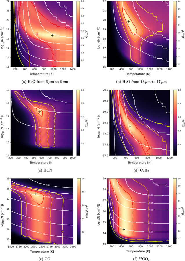
Figure 7. Reduced χ2 maps resulting from the fitting of LTE slab models to the MIRI MRS spectrum. The colors indicate the  value, with 1 being the best-fit model. The white contours show the emitting radius in au, and the red, orange, and yellow contours show the 1σ, 2σ, and 3σ confidence intervals. The location of the best-fit models in the parameter space is shown by a black plus sign.
Download figure:
Standard image High-resolution image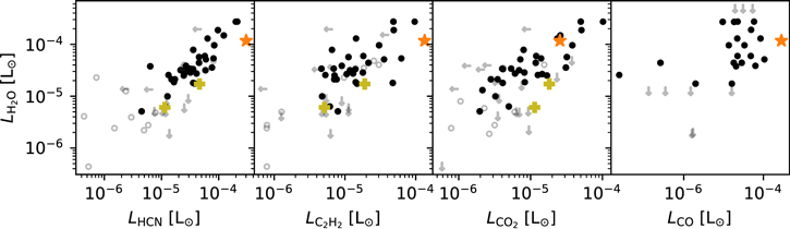
Figure 8. Comparison between the gas line luminosities of XUE 1 and the Spitzer sample studied by Banzatti et al. (2020) and the CO emission from Banzatti et al. (2022) (black circles). The y-axis shows the 17 μm H2O luminosity. From left to right the x-axis shows the 12CO2, HCN, C2H2, and CO luminosities. The upper limits are indicated with gray arrows, and the open circles show the sources with upper limits in both the x- and y-axes. The yellow plus signs show the location of the MIRI spectra published to date: GW Lup (Grant et al. 2023) and EX Lup (Kóspál et al. 2023). The luminosities measured for the JWST spectrum of XUE 1 are shown with the orange stars.
Download figure:
Standard image High-resolution image
Finally, we note that XUE 1 was also detected as an X-ray source in a Chandra observation (Townsley et al. 2019). The inferred X-ray column density  cm−2 and X-ray luminosity
  erg s−1 are consistent with the source extinction of AV
∼ 9 mag and mass of M ∼ 1 M⊙ for the more massive A1 component. This is a quite typical value for a young, approximately solar-mass star.
erg s−1 are consistent with the source extinction of AV
∼ 9 mag and mass of M ∼ 1 M⊙ for the more massive A1 component. This is a quite typical value for a young, approximately solar-mass star.
Appendix B: Distance of XUE 1
XUE 1 is located near the center of the stellar cluster Pismis 24. Since no parallax information is available for XUE 1, we derived estimates of the mean distance to the Pismis 24 cluster in the following way:
For an initial, rough, and preliminary estimate of the distance to the NGC 6357 region, we compiled a list of 61 early-type stars (spectral types O and B0–B3) from the literature (Broos et al. 2013; Townsley et al. 2014; Russeil et al. 2017; Ramírez-Tannus et al. 2020; Russeil et al. 2020), identified their Gaia DR3 (Gaia Collaboration et al. 2016, 2023) counterparts, corrected their parallaxes according to Lindegren et al. (2021), and computed the maximum likelihood estimate for the mean distance of this sample. This yielded an initial estimate of 〈D〉(NGC 6357) = 1.663 ± 0.009 kpc; this value was used as prior information in the following steps of our distance determination.
Next, we defined the Pismis 24 cluster region as a 4 5-radius circle centered on the apparent center of Pismis 24 at
 ![$(\alpha ,\delta )[J2000]=({17}^{{\rm{h}}}{24}^{{\rm{m}}}43\buildrel{\rm{s}}\over{.} 0,-34^\circ 12^{\prime} 23^{\prime\prime} )$](https://content.cld.iop.org/journals/2041-8205/958/2/L30/revision1/apjlad03f8ieqn11.gif) . This region contains 21 of the O–B3 stars. We also collected a sample of X-ray-selected objects in the same region from Townsley et al. (2019) and could identify Gaia DR3 counterparts for 376 of these.
. This region contains 21 of the O–B3 stars. We also collected a sample of X-ray-selected objects in the same region from Townsley et al. (2019) and could identify Gaia DR3 counterparts for 376 of these.
In the next step, we checked for the presence of possible foreground and background stars in our two samples and excluded all stars for which the 3σ distance interval (i.e., [ 1/(ϖ + 3σϖ
), 1/(ϖ − 3σϖ
)]) lies outside the distance interval of 1.663 ± 0.1 kpc. This led to exclusion of one foreground star (2MASS J17244754–3415069, B1V,  pc) among the O–B3 stars and 13 foreground and 8 background objects among the X-ray-selected objects.
Finally, the mean distance to Pismis 24 was determined with the Bayesian inference code Kalkayotl by Olivares et al. (2020), using a Gaussian prior distance of 1.663 ± 0.1 kpc. For the O–B3 stars this yielded 〈DOB3〉 = 1.687 kpc with a central 68.3% quantile (1σ distance interval) of [ 1.648, 1.726 ] kpc, and for the X-ray-selected sample we found 〈DX〉 = 1.694 kpc with a central 68.3% quantile of [ 1.656, 1.732 ] kpc. Since these two distance estimates for the OB and the X-ray-selected stars in Pismis 24 are very well consistent, we use D ≃ 1.69 kpc as the best estimate for the mean distance of Pismis 24 and thus for XUE 1.
Appendix C: Spectral Analysis
In the following we describe the analysis procedure to derive the properties of the molecular species identified in the spectrum of XUE 1.
C.1. CO Fundamental
The MIRI spectrum contains a part of the P-branch of the CO fundamental. Both the v = 1 − 0 and the v = 2 − 1 rovibrational transitions are detected in the spectra. In this section we present a first approach at deriving the excitation temperatures via the population diagram method (Goldsmith & Langer 1999), and we determine the temperature, column density, and emitting area by means of fitting non-LTE slab models to the spectra.
C.1.1. Rotation Diagram
We selected the lines to be fitted by visually inspecting the spectrum and picking only those lines in which the v = 1 − 0 and v = 2 − 1 transitions are resolved and not contaminated by H2O. We fitted the v = 1 − 0 corresponding to upper J levels between 24 and 33 and Jup = 46 and v = 2 − 1 with upper J levels between 18 and 28 excluding Jup = 23 and including Jup = 41. We determined the flux of each line and the continuum level by simultaneously fitting a zero-degree polynomial and all the selected lines with Gaussian profiles. To do the Gaussian fits, we assumed an error of 10−4 Jy, which corresponds to the typical error of line-free regions. The errors in the line fluxes (reported in Table 2) were calculated as the square root of the covariance matrix. The specific intensity, I, was determined by integrating over each profile and dividing the observed flux by the solid angle, Ω, assuming an emitting area of 0.5 au and a distance to XUE 1 of 1690 pc. The column density was then calculated using the formula
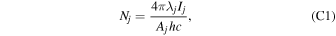
where λ is the central wavelength of each transition, Aj is the Einstein A-coefficient of each transition, h is the Planck constant, and c is the speed of light. Assuming that CO is in LTE, the energy levels can be described by a Boltzmann distribution. We can therefore express the relative column densities of any two excitation levels in terms of an excitation temperature Tex as
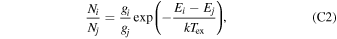
where gj
is the statistical weight of the rotational level, Ej
is the energy of the upper level, and k is the Boltzmann constant. The excitation temperature Tex corresponds to the inverse slope of the  versus Eup relation.
Table 2. Measured Fluxes of the CO Fundamental Lines Used for the Rotation Diagram and the CO χ2 Modeling (Section 3.1)
| Wavelength | vup | Jup | Flux |
|---|---|---|---|
| (μm) | (10−16 erg s−1 cm−2) | ||
| 5.1887 | 1 | 46 | 1.853 ± 1.135 |
| 5.1192 | 1,2 | 41,36 | 3.158 ± 0.889 |
| 5.1057 | 1,2 | 40,35 | 3.551 ± 0.933 |
| 5.0924 | 1,2 | 39,34 | 3.814 ± 0.945 |
| 5.0792 | 1,2 | 38,33 | 3.443 ± 0.91 |
| 5.0661 | 1,2 | 37,32 | 3.942 ± 0.96 |
| 5.0532 | 1,2 | 36,31 | 3.871 ± 0.919 |
| 5.0405 | 1,2 | 35,30 | 3.907 ± 0.989 |
| 5.0279 | 1,2 | 34,29 | 2.971 ± 0.919 |
| 5.0154 | 1 | 33 | 3.286 ± 0.911 |
| 5.0031 | 1 | 32 | 4.318 ± 0.945 |
| 4.9908 | 1 | 31 | 3.998 ± 0.907 |
| 4.9788 | 1 | 30 | 4.979 ± 0.933 |
| 4.9668 | 1 | 29 | 4.602 ± 0.933 |
| 4.9550 | 1 | 28 | 4.785 ± 0.925 |
| 4.9434 | 1 | 27 | 4.461 ± 0.884 |
| 4.9318 | 1 | 26 | 4.205 ± 0.904 |
| 4.9204 | 1 | 25 | 4.89 ± 0.901 |
| 4.9091 | 1 | 24 | 6.379 ± 1.036 |
| 5.1855 | 2 | 41 | 0.518 ± 0.941 |
| 5.0184 | 2 | 28 | 0.778 ± 0.932 |
| 5.0065 | 2 | 27 | 0.515 ± 0.761 |
| 4.9947 | 2 | 26 | 1.015 ± 1.042 |
| 4.9831 | 2 | 25 | 0.768 ± 1.054 |
| 4.9716 | 2 | 24 | 1.193 ± 1.122 |
| 4.9490 | 2 | 22 | 0.918 ± 0.871 |
| 4.9379 | 2 | 21 | 0.777 ± 0.892 |
| 4.9269 | 2 | 20 | 1.373 ± 1.021 |
| 4.9161 | 2 | 19 | 1.211 ± 0.827 |
| 4.9054 | 2 | 18 | 1.194 ± 0.912 |
Note. The blended lines (excluded from the rotation diagram) are indicated by listing both vup and Jup levels.
Download table as: ASCIITypeset image
C.1.2. Non-LTE Slab Models for CO
The ratio between the CO v = 1 − 0 and the v = 2 − 1 emission lines in XUE 1 is particularly high and cannot be reproduced by LTE slab models. We therefore opt to fit the observed CO spectra with radex non-LTE slab models (van der Tak et al. 2007) using the molecular data from Song et al. (2015). We follow the methodology from Tabone et al. (2023); we assume the line profiles to be Gaussian with a broadening ΔV = 4.7 km s−1 as in Salyk et al. (2011). In the non-LTE models the density of collision partners n<H> is a free parameter, allowing us to decrease it in order to match the line ratio between the fluxes of the v = 1−0 and v = 2−1 lines. The collision partners are H2, He (0.1n<H>), and electrons (10−5
n<H>). Other free parameters are the column density (NCO), the excitation temperature (Tex), and the emitting area given by  , where Rdisk does not necessarily correspond to the disk radius but could also represent a ring with the same area. Further studies are needed to account for the effect of fluorescence, which can also affect the v = 1 − 0/v = 2 − 1 line ratio, but this is beyond the scope of this paper.
We fit the CO v = 1 − 0 upper J levels between 24 and 41 and Jup = 46 and v = 2 − 1 with upper J levels between 18 and 36, excluding Jup = 23, where the lines with Jup between 29 and 36 are blended with the v = 1 − 0 lines with Jup between 34 and 41 and Jup = 41. We use a χ2 minimization to find the best model that adjusts to the observations. We compared the fluxes derived in Section C.1.1 with their respective errors to the model fluxes.
In an optically thin regime, NCO and Rdisk would be degenerate. Therefore, we can take advantage of the resolution of JWST in order to get an extra constraint on the emitting radius. We measure the width of the individual transitions and assume that the extra line broadening is due to Keplerian rotation. The projected rotational velocity can be expressed as

where i is the angle at which we observe the disk and  . Here FWHMinst is the expected line width due to the resolution of the instrument (R ∼ 4000; Argyriou et al. 2023), and FWHMobs is the measured line width. The resulting velocity can then be used to provide additional constraints on the emitting surface radius provided that we know the mass of the central star, allowing us to circumvent the degeneracy between the column density and the emitting surface radius.
Table 3. Overview of the Parameter Ranges for the Modeling Procedure
| Species |

| T | Fitting Ranges |
|---|---|---|---|
| (cm−2) | (K) | (μm) | |
| H2O @7 μm | 15–22 | 100–1400 | 6.404–6.422 |
| 6.445–6.456 | |||
| 6.467–6.478 | |||
| 6.630–6.641 | |||
| 6.678–6.689 | |||
| 6.781–6.792 | |||
| 6.858–6.871 | |||
| 7.039–7.051 | |||
| 7.202–7.212 | |||
| H2O @15 μm | 15–22 | 100–1400 | 13.498–13.507 |
| 14.173–14.182 | |||
| 14.205–14.215 | |||
| 14.322–14.332 | |||
| 14.341–14.350 | |||
| 14.402–14.412 | |||
| 14.422–14.432 | |||
| 14.482–14.493 | |||
| 14.820–14.830 | |||
| 14.880–14.899 | |||
| 15.050–15.060 | |||
| 15.178–15.187 | |||
| 15.324–15.332 | |||
| 15.341–15.353 | |||
| 15.412–15.423 | |||
| 15.450–15.460 | |||
| 15.564–15.574 | |||
| 15.621–15.631 | |||
| 15.720–15.763 | |||
| 15.790–15.808 | |||
| 15.962–16.015 | |||
| 16.105–16.120 | |||
| 16.217–16.227 | |||
| 16.271–16.274 | |||
| 16.317–16.327 | |||
| HCN | 14–19 | 200–1000 | 13.980–13.997 |
| 14.022–14.057 | |||
| 14.290–14.308 | |||
| C2H2 | 17–20 | 100–1200 | 13.562–13.748 |
| 12CO2 | 13–19 | 100–1400 | 14.932–14.940 |
| 14.959–14.990 | |||
| CO | 14–20 | 100–3400 | 4.900–5.152 a |
| 5.18–5.19 |
Note.
a See Appendix C.1.2 for the list of lines used.Download table as: ASCIITypeset image
C.2. LTE Modeling of H2O, HCN, C2H2, and 12CO2
In order to characterize the remaining molecular emission features present in the spectrum of XUE 1, we model them with the LTE model presented in Tabone et al. (2023), which has also been used in Grant et al. (2023), Perotti et al. (2023), and Gasman et al. (2023). We included emission from H2O (around 7 and 15 μm), 12CO2, 13CO2, OH, C2H2, and HCN, with molecular data from the HITRAN database (Gordon et al. 2022). As with CO, Gaussian intrinsic line profiles with ΔV = 4.7 km s−1 are assumed. For the HCN and 12CO2
Q-branches, we included mutual shielding from adjacent lines as described in Tabone et al. (2023). Under the LTE assumption we are able to fit the data with three free parameters: the gas temperature T, the column density N, and the emitting area as parameterized by an emitting radius Rdisk ( ). As in the case of CO, Rdisk is not necessarily the disk radius but could also represent a ring.
In order to fit the MIRI MRS spectrum, we first subtract the continuum locally by selecting line-free regions (see Table 3). We fit a spline function to determine the continuum level and subtract this from the MIRI spectrum. We then proceed to fit individual regions of the spectrum containing different molecules following a similar procedure to that described in Grant et al. (2023).
For each molecule, we ran a grid of models varying N in steps of 0.166 in  -space, T in steps of 25 K in linear space, and Rdisk from 0.01 to 10 au in steps of 0.03 au in
  -space. The best-fitting models were found by means of a χ2 fitting procedure. We measured the typical error in the flux in several line-free regions of the spectrum and adopted an error of 10−4 Jy for the wavelength range between 13 and 17 μm. We convolved the model spectra with a resolution R = 3000 for the water around 7μm and with R = 2500 between 13 and 17 μm to mimic the limited spectral resolution of MIRI MRS. We then resampled the convolved model to the wavelength grid of the observations. The χ2 was calculated at given spectral regions in order to avoid regions of the spectrum that are strongly contaminated by other species while still including lines that are sensitive to temperature and optically thin lines. In the case of H2O we selected the regions in which to calculate χ2 by running an LTE model with T = 800 K, N = 1017 cm−2, and R = 1 au to identify the spectral region where strong water lines are expected around 7 and 15 μm. The parameter ranges, as well as the wavelength regions used to calculate the χ2, are listed in Table 3.
To further reduce the contamination by other species, we follow the iterative procedure described in Grant et al. (2023). In short, we first fit H2O, subtract the best-fitting model from the continuum-subtracted data, and then proceed to do the same for HCN, C2H2, and 12CO2. We then subtract the composite best model of HCN, C2H2, and 12CO2 from the data and repeat the procedure for H2O. We perform this process once and find no change in the best parameters, nor any improvement on the residuals.
Appendix D: Reduced χ2 Maps
The reduced χ2 maps for H2O (around 7 μm and 15 μm), HCN, C2H2, 12CO2, and CO are shown in Figure 7.
Appendix E: Comparison of Line Luminosities with Other Samples
Figure 8 shows the line luminosity of H2O, measured from the 17 μm lines, against the HCN, C2H2, 12CO2, and CO of XUE 1 in comparison with a sample of T Tauri stars located in nearby (<200 pc), young (1−3 Myr) star-forming regions from Banzatti et al. (2020, 2022) and the newly obtained JWST observations of isolated PPDs (Kóspál et al. 2023; Grant et al. 2023).