
Abstract
The Nationally Determined Contributions pledged by numerous countries under the Paris Climate Agreement refer to efficiency gains as a key instrument for achieving carbon emission reductions. Indicators for estimating emission savings from resource efficiency projects can play a key role in identifying and prioritising projects. Building on existing emission factor-based approaches, this paper introduces a methodology which allows consistent ex-ante estimation of lifetime carbon savings from corporate resource efficiency investments. This methodology accounts for the intertemporal dimension of resource savings and project lifetimes and allows consistent aggregation across resource and project types. Moreover, it shows how social benefit (or cost) can be monetised. The methodology is tested using a resource efficiency investment project under the UN Clean Development Mechanism. We demonstrate that this indicator can be a robust, coherent and practical tool for firms, governments and investors to estimate carbon emission reductions from resource efficiency investments.
1 Introduction
By June 2017, 145 countries had submitted outlines of their climate change mitigation strategies as part of their Nationally Determined Contributions (NDCs) to the United Nations Framework Convention on Climate Change (UNFCCC) agreement reached in Paris. These NDCs specify the policy instruments and priorities that each country identified to be viable and suitable given the country’s specific socio-economic conditions. Following the adoption of the agreement, the key challenge for governments is to translate pledged commitments into concrete policy measures.
Aside from expanding renewable energy capacity, plans to increase resource efficiency—and energy efficiency in particular—are a key policy component in at least a third of all submitted NDCs (IEA 2015). This is especially the case for the commitments by large low- and middle-income countries, including India, China and Nigeria. The International Energy Agency (IEA 2015) estimates that the pledged energy efficiency improvements alone will require investments of $13.5 trillion globally between 2015 and 2030. This figure is likely to be significantly larger when considering investments in not only energy efficiency, but resource efficiency more generally.Footnote 1 While there is a clear focus on energy efficiency, it is important to recognise that not only emissions are associated with energy, but they can be “embodied” or triggered by materials (Denis-Ryan et al. 2016) such as carbon emissions from steel production or methane emissions from land filling materials (Ekins et al. 2016). For achieving ambitious emission reductions and for increasing economic competitiveness, it is thus critical to direct efforts not solely to increasing energy efficiency, but resource efficiency more broadly (UNEP IRP 2011).
While governments can provide a conducive environment to incentivise and support investments in efficiency, the identification and implementation of concrete investment projects are typically up to end-users, such as firms and households (Fay et al. 2015). Particularly the energy sector, and energy- and resource-intensive firms will play a key role in implementing investment projects to increase resource efficiency (IEA 2014). Against this background, it is critical for firms and institutional investors (including multilateral development banks (MDBs) and infrastructure investment banks) to adopt a robust and coherent approach for assessing the greenhouse gas (GHG) emission reductions from resource efficiency investments (World Bank 2015). This can inform the selection of resource efficiency investments and help benchmark firm-level performance against national climate change mitigation and resource efficiency targets.Footnote 2
Instead of complex, convoluted and case-specific methodologies, this paper presents a GHG indicator which enables consistent ex-ante project appraisal. It extends existing frameworks by additionally accounting for cumulative emissions throughout a project’s lifetime, as well as one-off upfront resource inputs, technology benchmarks and a baseline scenario. Thus, the indicator can be used as a tool to estimate the overall net emissions impact of a future resource efficiency investment project.
The presentation and discussion of the GHG indicator in this paper put a particular focus on application in practice. It argues that more comprehensive approaches (such as life cycle analyses) have excessive data requirements which disqualify them from widespread and coherent application, especially in developing countries and small- and medium-sized enterprises (SMEs). Furthermore, the GHG indicator presented in this paper allows for the aggregation of savings across various resource types and investment projects. By allowing for disaggregated time series across project lifetimes, it is also better equipped to capture the intertemporal dimension of resource and emission savings (compared to existing approaches, e.g. by MDBs, which only consider average data for a “representative year”).
This paper further provides a comprehensive overview of relevant data sources which are required for applying the indicator to specific resource efficiency investment projects, and offers a case study example to highlight potential challenges—and solutions—for application in practice. Moreover, the GHG indicator will be linked with estimates of the “social cost of carbon” to monetise the social benefit (or cost) of a given investment, using standard discounting methods.
2 Existing frameworks for estimating emission savings of resource efficiency projects
Spurred by the signing of the UNFCCC in 1992 and the Kyoto Protocol in 1997, the establishment of market-based incentives for GHG emission reduction projects under the Clean Development Mechanism (CDM) has led to the development of a plethora of GHG emissions accounting frameworks (Ascui and Lovell 2011). These accounting frameworks are designed to estimate GHG emissions at a variety of levels, including national-, corporate-, project- or product-specific levels (Brander 2015; DEFRA 2009; BSI 2011).Footnote 3
This section outlines common approaches to estimating GHG emissions as well as the relevant literature. Starting from the broader concept of life cycle analysis (LCA), this section reviews how—in theory—the accurate estimation of GHG emissions requires a complete analysis along the entire life cycle associated with individual resources (Brander 2015; Ascui 2014; UNEP 2011). This section also discusses the emission factor approach, which is a derivation and simplification of the LCA methodology and thus the most commonly used approach in practice. In reviewing these methodologies, the section highlights methodical aspects relevant for ex-ante appraisal of resource efficiency projects.
2.1 Consequential life cycle analysis
In principle, a LCA aims to measure all environmental, economic and social impacts throughout a product’s entire life cycle and is thus able to reflect not only direct effects, but also indirect effects along supply chains (UNEP 2005; EU JRC 2012; Finnveden et al. 2009). While the classical LCA set-up provides a snapshot at a given point in time, consequential LCA measures how a change in certain exogenous parameters can affect environmental impacts (Weidema 1993). By analysing the change in material, product and elementary flows, consequential LCA is of particular interest for ex-ante assessment or ex-post evaluation of policy measures and corporate projects (Ekvall and Weidema 2004; McManus and Taylor 2015).
The International Organisation for Standardisation (ISO) sets out detailed principles for conducting LCAs (ISO 2006c). According to the ISO, a full-fledged LCA should include acquisition of raw materials, manufacturing, distribution and transportation, production and use of fuels, process electricity and heat, disposal of waste, use and maintenance of final products, possible recycling and reuse, and various other domains which are directly part of or affected along the life cycle. In theory, different LCAs would always take into account all these life cycle stages and thus be comparable.
However, in practice this analysis comprises a complex and large network of processing units and materials and may involve multiple causal circles—thus creating enormous data requirements. In this context, LCAs and life cycle inventories more generally rely on the extrapolation of market trends and estimates from various economics models including partial or general equilibrium simulations (Brander et al. 2008; Earles and Halog 2011). Consequential LCA, the most relevant LCA approach for ex-ante project appraisal, requires detailed knowledge on the nature of interaction between process units at the margin, i.e. marginal effects, and how these cumulate over time (Weidema 1999). Primary data on such marginal effects are particularly difficult to obtain in practice (Brander et al. 2008; Tillman 2000).
In face of stringent data requirements, more flexible consequential LCAs have been devised that allow for different system boundaries and degrees of depth. However, even very light versions of Consequential LCAs are still methodologically complex and time intensive, making them ill-suited for commercial appraisals of corporate resource efficiency investments (UNEP 2005). This is particularly true for SMEs or developing-country settings where data availability remain an obstacle. More importantly, while flexible and light consequential LCA methodologies sometimes make analysis feasible, results will lack comparability across firms as data limitations and system boundaries are case specific.
2.2 Emission factor-based calculations
Besides LCAs, emission factor (EF)-based calculations are the second main category of approaches relevant to estimating emission savings from resource efficiency projects (UNEP 2011). In its essence, this approach determines relevant activities (including resource usage and other operation features) and multiplies these with EFs which reflect the embodied GHG emissions associated with the activity (DEFRA 2009). Over the past two decades, EF-based approaches have been adopted widely and feature in various product-, project-, firm- and national-level GHG accounting guidelines, as well as analytical models (e.g. BSI 2011; ISO 2006b; IPCC 2006; van Voet et al. 2005).Footnote 4
The accuracy of EF-based approaches necessarily depends on the quality and suitability of emission factors used. Emission factors reflect the average GHG emissions associated with specific process activities or inputs (ISO 2006b). Such factors are often estimated by applying LCA techniques, or processing data from national GHG inventories (DEFRA 2015; EPA 2016). Various databases exist that compile a large number of specific emission factors, which typically reflect GHG flows originating from a defined set of process units and relate them to corresponding energy, material or product flows (see Sect. 3.1).
While existing EF databases provide a rich source of reference, it must be recognised that these emission factors are an approximation and thus imprecise under any case-specific circumstances. Similarly, emission factors can also not accurately inform about marginal patterns, which depend on case-specific parameters (Ekvall and Weidema 2004). Nevertheless, Brander et al. (2008) suggest that average data may serve as a reasonable approximation, especially if project interference is small relative to sectoral economic activity (Yang 2016).
The availability of detailed EF databases and the relative simplicity of application has led to EF-based methodologies being applied far more frequently in practice than LCA. For instance, acknowledging data availability in developing countries, CDM projects frequently approved methodologies that resort to EF techniques (Ascui and Lovell 2011). ISO 14064-2 on the “quantification, monitoring and reporting of GHG emission reductions” also explicitly refers to EF as a means to calculate emissions (ISO 2006b; Brander 2015). Similarly, the European Investment Bank (EIB) also applies an EF-based methodology to assess the GHG emission impacts of their investment projects (EIB 2014).
Besides their applicability under major data constraints, another critical advantage of emission factors is the coherence and comparability of results. Since emission factors are based on a pre-defined scope of analysis (i.e. considering a set life cycle segment, such as “cradle-to-gate”), using the same emission factor across different projects means that the scope of analysis remains consistent.
2.3 Ex-ante project appraisal: accounting for the time dimension of GHG emissions
The standard GHG accounting frameworks outlined above typically do not account for potential variations in GHG emissions throughout a project’s lifetime. This makes these accounting frameworks suitable for the purpose of continuous performance monitoring (e.g. for annual reporting), but not necessarily for the ex-ante appraisal of GHG mitigating investments, such as those in energy and material efficiency. Such projects typically mitigate emissions throughout long project lifetimes, with possibly large variations in different years of operation.
The EIB partly addresses this issue by factoring in a project’s expected lifetime, and the estimated average GHG savings from a “typical year of operation” following an investment (EIB 2013, 2014).Footnote 5 Moreover, it applies social cost factors (i.e. a “shadow carbon price”) to estimated emission savings in order to integrate external costs into the profitability analysis. While this approach is more suited to the purpose of ex-ante project assessment, it still neglects information on the point of time of emissions. Similarly, while consequential LCA accounts for net intertemporal effects, it does not assign them to explicit points in time (Brander 2015). Especially for considering GHG emission reduction projects, the timing of emissions can play a crucial role in determining the associated social benefits or costs (Hope and Johnson 2012).
Investment appraisals of resource efficiency projects typically estimate time series of resource savings by distinguishing between intervention and baseline scenarios, thus allowing the calculation of resource savings for any given year of the project’s lifetime (Brander 2015). The methodology presented in the following section makes use of this information in order to estimate embodied emission savings from a variety of resources across time and to allow incorporating the associated social benefits into conventional commercial project appraisals.
3 Ex-ante estimation of GHG emission savings from corporate resource efficiency investments
There are three key objectives of the GHG emissions indicator presented in this paper.
- 1.
Coherently estimating net emissions savings of firm-level resource efficiency investments.
- 2.
Allowing for dynamic benchmarking and taking into account the time dimension of resource savings over project life times.
- 3.
Allowing savings to be aggregated across various resource types and investment projects.
This can assist firms, governments and investors in assessing the performance of investment projects in terms of GHG emissions intensity and compare firm-level performance against national targets on efficiency gains and emission reductions. In particular, this indicator encompasses direct and embodied GHG emission savings associated with energy and material efficiency.
This focus on applicability requires this GHG emissions indicator to reconcile a robust methodology with potentially limited data availability. Data constraints and limited monitoring capacity at the firm-level may obstruct such coherence and thus be a particular challenge for firms in developing economies as well as SMEs. Taking this into account, the indicator presented in this paper uses a standardised calculation procedure, which requires relatively little primary data and relies on emission factors available from existing databases.
The GHG emissions indicator presented in this paper builds on existing GHG accounting principles which are already in use (e.g. the UK’s guidance on how to measure and report corporate GHG emissions; DEFRA 2016) and adds a time dimension. Existing GHG accounting frameworks are intended as “snapshot” indicators of total current observed emissions; by calculating these indicators on a regular (usually annual) basis, performance can be monitored and tracked over time. However, by considering cumulative lifetime emissions, one-off upfront resource inputs, as well as a baseline scenario and technology benchmarks, the GHG indicator in this paper enables ex-ante project appraisal—i.e. it can be used as a tool to estimate the overall net emissions impact of a future resource efficiency investment project. Notably, it allows to account for general technological progress, e.g. by dynamically comparing the project’s output emission intensity to industry averages at each point in time.
The remainder of this section outlines the information requirements (Sect. 3.1), a theoretical exposition of the indicator’s conceptual framework (Sect. 3.2) and a discussion of how estimated GHG savings can be monetised to reflect the societal net benefit of a resource efficiency project (Sect. 3.3).
3.1 Information requirements
The methodology has, similar to all EF-based calculations, the following two main information requirements for estimating GHG emissions from energy and material efficiency investments.
- 1.
Resource savings The types and quantities of energy and materials savings, and at which point in time these occur. If general technological advances are expected, benchmark emission intensity has to be adjusted over time accordingly.
- 2.
GHG emission factors The GHG emission factors associated with different types of energy and materials savings.
3.1.1 Energy and material savings
Estimating GHG emission savings requires quantitative information on the projected energy and material consumption of a given investment project as compared to an appropriate benchmark. This data requirement consists of (1) the specific types of energy and material, (2) the quantities for each resource type, (3) the point in time when these savings will occur and (4) information about emission intensity at which the economy would provide the same output without the investment.
The specific types of energy (e.g. natural gas, oil, electricity) and material savings (e.g. metals, plastics, minerals, biomass) need to be identified to enable coherent matching with the relevant GHG emission factors, as described in the next subsection. The quantities are required in order to multiply them with the GHG emission factor. Moreover, to compare the monetary benefits of GHG savings over time, it is crucial to determine at which specific point in a facility’s lifetime the savings occur. Even if the absolute consumption of energy and materials is unknown, only the changes in energy and material use are required to calculate the resulting GHG emission savings.
3.1.2 GHG emission factors
In line with other indicators within the emission factor-based methodology, the proposed approach considers GHG emission factors to calculate the GHG emission savings of efficiency investments. GHG emission factors provide information on the CO2e emissions of the aggregated supply chain of energy and materials across their life cycle or until the firm’s gate (cradle-to-gate). In other words, individual life cycles of resources are approximated by the average life cycle of that resource, which is often calculated for a particular country. In practice, data limitations mean that not the entire life cycle is covered.
Several databases of empirically estimated GHG emission factors exist. Table 1 presents the most comprehensive databases which are publicly available and discuss their coverage and scopes.
The Inventory for Carbon and Energy (ICE) database comprises GHG emission factors of over 200 common industrial materials (Hammond and Jones 2011). It covers primary and secondary raw materials and takes the UK industry fuel mix and recycling rates as benchmarks. The database is compiled from secondary sources by the University of Bath. The ICE database follows a coherent set of criteria that ensure data quality and comparability across materials. However, due to data constraints, some GHG emission factors underlie heterogeneous boundary conditions. The database’s focus is on industrial materials; thus, it might not cover all materials of interest.
The Kreditanstalt für Wiederaufbau (KfW) uses a relatively well-endowed database of EF for approximately 160 industrial primary and secondary materials as well as agriculture products. For the majority, considered life cycle stages are explicitly stated. Figures result from a study conducted by the Institute for Energy and Environmental Research Heidelberg which is also included in the PROBAS database.
The DEFRA Conversion Factors for Company Reporting compiled by the private consultancy Ricardo-AEA for the Department for Environment, Food and Rural Affairs (DEFRA) are tailored to depict emissions caused by business activities, especially within the UK. They augment a broad spectrum of corporate processes with direct, i.e. single activity, and indirect emission, i.e. equivalent to cradle-to-gate, and contain cradle-to-gate emissions for selected construction materials, metals, paper, plastics and electrical items. Although derived from a variety of sources, consistent treatment and annual updates ensure quality and coherence among the figures provided.
Recently revised and partly updated by the providing German Federal Office for the Environment (Umweltbundesamt), the PROBAS database collects detailed life cycle inventory (LCI) data including figures of different and aggregated (CO2e) GHG emissions for various processes, fuels, secondary energy sources and materials. Sometimes multiple entries are available for the same material or process. Where appropriate, environmental pressures account for upstream processes, thus providing cradle-to-gate EF. Much of the data are sourced from research institutes, including Öko-Institut Freiburg and IFEU Heidelberg. Geographical and temporal boundaries are heterogeneous.
The IPCC’s Emission Factors Database (EFDB) aims to supply default data for every possible GHG-emitting process within the economy. Comprehensive guidelines and data set descriptions accompany the usage. Note that their EF never incorporate emissions beyond those resulting from the single process they are assigned to. However, the EFDB comprises probably the most common emission factors that are often employed to construct EF of larger scopes.
The Canadian Raw Material Database, compiled and maintained by the University of Waterloo, Ontario, reports life cycle inventory data for environmental input and outputs of materials processed in Canada. Although a small data set, figures are supposed to provide reliable information for industrialised economies in general due to diligent maintenance. No secondary sources were in use.
The Athena Sustainable Materials Institute supplies a small software package, which enables the user to account for GHG emissions from construction activities, including those emissions from processing, transport and demolition of the materials. Although the underlying database is not readily available, EF can be extracted for single materials or a mixture from the software output. Furthermore, it facilitates the assessment of on–off emissions from commissioning. Emissions at different stages are presented separately, thus allowing for individual scope assembly. The LCI data, which result from own analysis, are said to be region-sensitive within the geographical boundary of North America.
3.2 Conceptual outline of the aggregated GHG indicator
In its essence, the indicator accounts for the projected resource savings of a given resource efficiency investment and aggregates the associated emission savings. It is important to adequately define the project boundaries for calculating the resource savings, i.e. which resource savings should be included or excluded from the indicator. Typically, the boundaries should reflect the direct business impacts of a project. Depending on project type, project boundaries may reflect (1) physical boundaries (e.g. a production plant) or (2) system boundaries (e.g. an electricity grid) and thus require case-by-case consideration.
Particularly in resource-intensive manufacturing firms, resource efficiency investments typically affect a range of material and energy inputs. As a first step, the indicator converts these various types of physical resource savings into respective emission savings, using relevant GHG conversion factors (see Sect. 3.1). As a second step, emission savings associated with different resource types are aggregated to obtain the overall net emission savings of the investment project. To maintain coherence and comparability, it is important to express quantities relative to the quantity or value of output.
This methodology can be formally expressed. As outlined in Sect. 3.1, the first information requirement is the consumption of resources per unit of output. Relative usage \(r_{t,n}\) of resource \(n\) at time \(t\) may be computed as \(r_{t,n} = R_{t,n} /Y_{t}\)—where \(R_{t,n}\) is absolute resource consumption and \(Y_{t}\) is output—while at tome data on resource input intensities may be easier to obtain than on absolute resource consumption in the first place. Resource savings are then defined as the difference between relative resource usage and a dynamic (i.e. time variant) benchmark \(r_{t,n}^{\text{B}}\):
The dynamic benchmark \(r_{t,n}^{\text{B}}\) is case specific and typically depends on the resource intensity of peer projects or industry averages. Typically, this involves assumptions about the future path of production technology, while in some cases a constant benchmark may be appropriate. The case study in Sect. 4.2 illustrates how a dynamic benchmark can be derived.
Defining \(T\) as the project’s total lifetime, aggregated savings for each resource \(n\) are obtained as:
Subsequently, aggregated savings \(\sum_{t} \Delta R_{t,n}\) are multiplied with the resource’s respective emission factor \(\varepsilon_{n}\) to obtain aggregated emission savings \(\Delta E_{n}\) corresponding emissions aggregated.Footnote 6
where \(N\) is the total number of resource types under consideration. Note that the change in emissions \(\Delta E_{n}\) associated with different resource types can be either positive or negative. Aggregating emission savings related to different resources yields the overall net emission savings \(\Delta E_{\text{total}}\). This aggregation yields a single number (or indicator) which reflects the total net change in emissions due to a resource efficiency investment.
In some cases, data constraints may make it necessary to benchmark against industry-level aggregate emission intensities\(e_{t}^{\text{B}}\) rather than \(n\) different resource-specific input intensities \(r_{t,n}^{B}\). For example, aggregate emission intensities can often be easily derived from existing studies, which in turn greatly reduces information requirements on the benchmarking. In such cases, one first computes the project’s emission intensity, for every point in time:
Then, benchmarking against \(e_{t}^{\text{B}}\), scaling by project output and aggregating over time yield total emission savings:
3.2.1 Accounting for changes to technology lifetime
In addition to capacity changes, the replacement of old machinery is likely to increase the operational lifetime of production facilities.Footnote 7 In other words, the post-investment lifetime of a plant is likely to extend beyond the original (baseline) lifetime. Savings vary for different assumptions on operational lifetime (e.g. when extending the lifetime of an existing facility). In principle, the impacts of an intervention should be estimated throughout the facility’s lifetime.
Figure 1 presents a hypothetical example to illustrate the role of increased capacity (hence output) and extended lifetime in the context of a resource efficiency intervention. The challenge for benchmarking emission savings is the fact that an investment may reduce resource usage per unit of output and thus relative emission intensity, but this gain may be offset by an increase in the production volume, thus resulting in an absolute increase of emissions.

Output and lifetime changes in a hypothetical production unit for (1) the baseline scenario (i.e. no investment) and (2) the projected investment scenario
Taking into account potential increases in production output and lifetime, two main scenarios can be distinguished with respect to post-investment emissions:
- 1.
Output increases exceed efficiency gains The absolute increase in production output (and thus resource use) offsets relative efficiency gains. While the emission intensity of a given unit of output is lower than in the baseline scenario, emissions are higher in absolute terms. This is aggravated by the fact that the extended lifetime means additional emissions (years 8–10 in this example). This scenario is illustrated in Fig. 2 and is a form of Jevon’s Paradox
Fig. 2 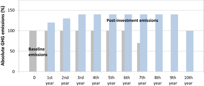
Resource-related emissions of a hypothetical firm: capacity increases offset any efficiency gains; thus, absolute emissions exceed baseline emissions. Grey bars depict baseline emissions (i.e. no investment). Blue bars depict emissions after a resource efficiency investment
- 2.
Efficiency gains exceed output increases In this case, the decrease in emission intensity of each unit of output is large enough to offset the additional emissions due to capacity increases. In other words, emission savings due to resource efficiency increase at a higher rate than output. Whether this translates into positive or negative absolute emission savings due to the investment depends on the extent to which lifetime is extended, i.e. referring to the example (Fig. 3), do emission savings in years 1–7 exceed additional emissions in years 8–10?
Fig. 3 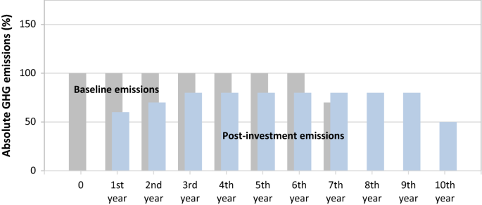
Resource-related emissions of a hypothetical firm: emission savings due to efficiency gains offset additional emissions due to output increase. Grey bars depict baseline emissions (i.e. no investment). Blue bars depict emissions after a resource efficiency investment


3.2.2 Accounting for one-off emissions
In addition to running emissions associated with ongoing production, certain resource efficiency investments may cause significant one-off emissions. This is particularly the case with green-field projects, but also with other modernisation projects requiring major construction activities. Such projects typically use large one-off inputs of energy and materials, which cause or embody significant GHG emissions before the new facility even becomes operational. If the material and energy use of such upfront one-off activities is indeed found to be significant, they must be added to cumulative resource savings (as negative savings).Footnote 8 Equation (3) is modified accordingly, to account for initial one-off resource use \(I_{n}\).
3.2.3 Benchmarking
Choosing an appropriate case-specific benchmark is critical for obtaining a robust and meaningful estimate of an investment’s emission savings (WRI/WBCSD 2005; Gustavsson et al. 2000). In particular, all post-investment output that exceeds baseline output needs to be evaluated against a chosen benchmark, which specifies technology and output levels in the absence of the considered intervention (Brander 2015). For this purpose, underlying assumptions are essential for determining an appropriate benchmark.
Zero benchmarking A conservative approach is to treat all additional output (i.e. capacity increases, depicted red in Fig. 1) and the associated emissions as purely additional. In other words, the underlying assumption is that without the investment, the firm would not increase its capacity, and after the end of the current expected lifetime (year 7 in Fig. 1) production would terminate and no replacement capacity installed. This approach of treating emissions as purely additional is likely to yield a conservative estimate of net emission savings.
Best available technology (BAT) An alternative to zero benchmarking is to use BAT as a reference point. BAT refers to the most efficient technology (locally or internationally) available to a given firm; in practice, this may also include locally used new technologies, or regional best performers. Comparing post-investment emission intensities of additional output (red in Fig. 1) against a BAT benchmark assumes that capacity increase and life extension would occur regardless of the investment using alternative technologies—for instance, as part of a general growth trend. Note that an investment can yield positive emission savings even if it underperforms compared to a BAT—as long as it outperforms the baseline scenario in terms of absolute emissions.
3.3 Social benefits: monetising an investment’s GHG savings
As savings across different types of resources are all converted into the common unit of tonnes of CO2e emission savings, it is possible to estimate the societal benefit of a given resource efficiency project in monetary terms. Monetising the social cost or benefit of emission savings relies on estimates of the so-called social cost of carbon. However, to obtain the net present value of social costs (or benefits), emission savings cannot simply be aggregated across time, but must be monetised—and discounted—year by year.
Estimates of the social cost of carbon (SCC) rely on long-term simulations in complex physical and economic systems and are thus necessarily associated with uncertainties. Notwithstanding, the use of SCC for assessing the social costs or benefits of investment projects is a common approach and adopted by the US government or the European Investment Bank (Hope and Johnson 2012; Interagency Working Group on Social Cost of Carbon 2013; Pindyck 2013; EIB 2013).
Formally, the SCC is equivalent to the net present value of cumulative (monetised) damages due to an additional tonne of CO2e. In principle, a tonne of carbon emitted in a given year \(t\) will cause damages for \(Y\) years; monetising, discounting and aggregating these damages yield an estimate of the SCC in year \(t\) values:
where \(\delta\) denotes the discount rate and \(D_{t + y}\) the monetised damages in \({\text{y}}\) years after time \({\text{t}}\). Note that immediate damages (i.e. \(y = 0\)) are not discounted. The US Interagency Working Group on the Social Cost of Carbon (2013) provides annual SCC estimates up until 2050, for different assumptions about the discount rate (see Appendix 1).
In line with previous notation, emission savings in year \(t\) can be expressed as resource savings (of different resource types) in year \(t\) multiplied by the relevant emission factor:
Figure 4 shows the overall annual emission savings (i.e. \(\varSigma_{i = 1}^{n} \Delta E_{t,i}\)) of the hypothetical resource efficiency investment throughout the operational lifetime of the plant.

Annual net emission savings, based on the scenario in Fig. 3
The nominal social cost (or benefit) \(n{\text{SCC}}_{t}\) associated with emission savings in year \(t\) from resource \(n\) is given by
Note that \(n{\text{SCC}}_{t}\) denotes the social costs (or benefits) from less (or more) resource efficient operations and is positive (i.e. a social benefit) for positive emission savings.
While more efficient operations save resources (and thus emissions), the investment project may require significant initial one-off resource use, thus causing emissions which must be accounted for. The social cost of such emissions due to the initial one-off usage of resource \(n\) can be written as
The social cost \({\text{SCC}}_{n}^{I}\) is negative if the project causes upfront initial resource use \(I_{n}\).
The project’s overall social cost (or benefit) \({\text{SCC}}\) is obtained by summing initial social costs \({\text{SCC}}^{I}\) and the running social costs for each year \(t\) of the plant lifetime. Initial social costs do not have to be discounted as they are in present values, while nominal social costs \(n{\text{SCC}}_{t}\) associated with emission savings in year \(t\) need to be discounted and transformed from year \(t\) into present values.
The social benefit (or cost) of emission savings (or additions) of overall resource savings in year \(t\) is shown in Fig. 5 (this corresponds to \(\sum\nolimits_{i = 1}^{n} {{\text{SCC}}_{t,i} }\)).

Social net benefit of emission savings due to the hypothetical resource efficiency investment. Monetised benefits are reported for discount rates of 2.5, 3 and 5% (see Appendix 1). For illustration purposes, the standardised emission savings in Fig. 4 are assumed to correspond one-to-one to tonnes of CO2e
4 Applying the methodology: case study
This section covers two issues. Firstly, it presents a practical application framework based on the formal GHG emission savings methodology (Sect. 3.2). Secondly, it applies the methodology to a case study, a resource efficiency project under the CDM.
4.1 A standardised application framework for policy analysts
Table 2 presents a standardised application framework, including the respective measurement units. The first column (“energy and material savings”) refers to cumulative resource savings of respective resource types aggregated across time, possibly including one-off resource inputs (denoted \(\sum_{t} \Delta R_{t,n} \mp I_{n}\) in Eq. (6)). The second column refers to the GHG emission factors associated with the specific resource type (\(\varepsilon_{n}\), see Sect. 3.1). The third column (“GHG emission savings”) corresponds to the emission savings associated with the various resource types (\(\Delta E_{n}\)). Before aggregating these separate emission savings, the application framework allows for double-counting adjustments. The reason for this is that in practice, project-specific circumstances and available information may cause component estimates to overlap. As this issue is entirely case specific, there is no standard approach for making double-counting adjustments. However, when applying the indicator, potential double counting in the source data needs to be accounted in order to reach a robust and coherent total GHG emission savings indicator (\(\Delta E_{n}\); rightmost column). With respect to the rows presented in Table 2:
Energy This category reflects the reduced use of different energy types, including grid electricity, or the on-site combustion of natural gas, coal, oil, etc., usually reported in MWh per year (MWh/y). Each energy type is treated separately to allow for different GHG factors across energy types and substitution among different energy types.
Materials This category allows for all types of materials, usually measured in tonnes per year (t/y). Again, each material type is treated separately.
4.2 Case study: UltraTech Cement Ltd
This section illustrates the application of the above framework for a resource efficiency project conducted under the CDM. The case study, UltraTech Cement Limited, is a large cement producer based in India supplying to both domestic and international markets (full project documentation from UNFCCC 2006). It operates various plants with total production of primarily grey cement of 69.3 million tonnes annually. In 2000, UltraTech Cement implemented a resource efficiency project at their facility in Tadipatri, southern India, which was credited by the CDM. The project aimed to save GHG emissions associated with the production of clinker by substituting lime with fly ash during the process of Portland Pozzolana Cement (PPC) blending.
4.2.1 Resource savings
Fly ash is a by-product, for instance, from coal-fired power plants, which is typically discarded as waste with various adverse side effects (e.g. water and soil contamination through land filling as well as coinciding costs of disposal). The production of clinker requires energy-intensive grinding and pyro-processing of raw materials, namely limestone and different additives. Throughout the production of clinker, GHGs are emitted during the calcination of limestone to lime and the combustion of fuels for heat and electricity. Savings were achieved on the second stage of production by substituting clinker with fly ash in blending the cement. In this project, resource use is reduced proportionally to the share of clinker in PPC production from 80.6 to 70.5%. Since other firms in the cement market are adopting similar measures to reduce their clinker inputs over time, the savings are not benchmarked against the initial clinker share, but rather against gradually declining average industry shares (UNFCCC 2006).Footnote 9
4.2.2 Data and assumptions
The official project document reports figures for cement production and clinker shares over the entire 10-year CDM-crediting period (UNFCCC 2006). Information on inputs, such as grid electricity, coal for heating and lime, is only available for the first 4 years. Hence, the missing data are approximated by applying average input ratios to data on clinker shares and total cement production, which in turn is provided for the total crediting period until 2010. The approximation bias is likely to be small due to stable input–output relations. In general, when choosing underlying assumptions and data, it should be kept in mind that moderate variations can significantly change final estimates quantitatively and qualitatively (Zisopoulos et al. 2016).
The plant considered in this case study draws electricity from three different sources, namely the Indian grid, a local gas-fired power plant and on-site combustion of coal. The utilisation ratios of the various types of electricity are derived from the provided data to estimate the respective input quantities.Footnote 10
Following UNFCCC (2006), the expected overall lifetime of the facility is estimated to be 25 years and thus exceeds the 10-year period monitored by the CDM. To derive emission savings for the total lifespan, the data are extrapolated based on two scenarios, designed to constitute an upper and lower bound for the assessment (graphical representation in Appendix 2).
The “Conservative Scenario” also keeps the project clinker share at 70.5%, but assumes no output increases beyond the last reported level. Furthermore, the baseline share does not depart from its initial trajectory at any point in time and will reach 68.5% in the last year of operation. Note that this results in negative net marginal emissions for the project.
The “Optimistic Scenario” assumes a maintained, linear increase in output until full utilisation, namely 2.3 million tonnes of PPC, while sustaining a clinker share of 70.5%.Footnote 11 The baseline clinker share follows its original trajectory, but does not undercut the project clinker share set at 70.5%.
Appropriate emission factors are drawn from the databases outlined in Table 1 in Sect. 3.1 and averaged for each type of input (in this case relevant figures were obtained mostly from the PROBAS database but also from the ICE and DEFRA tables; Sect. 3.1). Since the project is about incrementally decreasing the clinker share in existing production facilities and processes, there are no meaningful one-off emissions. For the purpose of this illustrative case study, each scenario assumes baseline output to be equivalent to the respective scenario’s output trajectory. This implies that the following results indicate the GHG savings of the proposed efficiency project, relative to an alternative project using less efficient technology.
4.2.3 Results
The results are summarised in Table 3 (conservative scenario) and Table 4 (optimistic scenario) for average emission factors. Table 3 presents the calculation of GHG emission savings over the facility’s total lifetime in case of no further output expansion, and continued decrease in the market clinker share (see Appendix 2). Given this scenario, the project saves approximately 1.03 million tCO2e in 25 years, thus just over 41,000 tCO2e per operational year. Almost 60% of the GHG emission savings stem from lime savings. Table 4 is based on the scenario of approaching full utilisation and a restricted increase in the baseline clinker share, which results in higher emission savings. The share of material savings of total GHG emission savings remains unchanged.
Figures 6 and 7 present the project’s annual GHG savings over time for both scenarios. Since the assumptions of the two scenarios concern the projection after 2010—i.e. when project documents provide no further information on output and the baseline clinker share—the graphs do not differ for the first 10 years.

Estimated CO2e emissions savings for the conservative scenario. The range is defined by the highest and lowest emission factors available in the EF databases

Estimated CO2e emissions savings for the optimistic scenario. The range is defined by the highest and lowest emission factors available in the EF databases
It becomes apparent that estimates are sensitive to the baseline clinker share, but less so to the evolution of output. When approaching 2021, output in the optimistic scenario is almost twice as high compared to the conservative setting, but GHG savings hardly differ. Moreover, considerable GHG “losses” after 2021 are to be attributed solely to different baseline clinker shares.
To illustrate the sensitivity of the analysis to variation of emission factors across different databases, calculations are repeated using the highest and lowest available emission factors from different databases (Sect. 3.1) to estimate a range; concrete estimates are based on average emission factors.
4.2.4 Estimating the social benefit
As outlined in Sect. 3.3, estimated GHG savings can be monetised as a measure of the social benefit (or cost) of a resource efficiency project. For this purpose, average GHG savings estimates in t CO2e are monetised based on the methodology in Sect. 3.3. The approach applies standard discount rates of 2.5, 3 and 5% as proposed by the US Interagency Working Group on the Social Cost of Carbon (2013). Figures 8 and 9 show the annual social benefit associated with the GHG savings of the case study project. It becomes apparent that the annual social benefits of GHG emission savings vary greatly depending on the discount rates. However, regardless of which discount rate or projection scenario is used, the results show that there are positive social net benefits from this investment project, i.e. this is the case even when considering the conservative project scenario and a relatively high discount rate.

Estimated monetised annual social benefit of emission savings in the conservative scenario

Estimated monetised annual social benefit of emission savings in the optimistic scenario
5 Discussion
The application of the GHG emission indicator to a resource efficiency project under the CDM has yielded several insights which are discussed in this section.
Intertemporal aspects matter The case study has shown that the common approach of considering an “average” post-intervention year is not adequate, considering only the first post-intervention year even less so, since the effects of efficiency investments require time to materialise. Material usage and thus emission savings can vary substantially from year to year throughout the project lifetime.
Sensitivity ranges are reasonable As the proposed indicator methodology has relatively low data requirements and relies predominantly on readily available data, the proposed GHG indicator has proven to be suitable for practical application. While the original project reports were designed to serve different methodologies, and thus omitted some data, carefully chosen assumptions have enabled results with reasonably narrow sensitivity ranges. For instance, the sensitivity analysis using confidence ranges for EFs yields savings trajectories, which are qualitatively similar. However, variations in the magnitude of annual savings highlight the importance of carefully selecting EFs. If data are available, local EFs can be used as they more adequately reflect the specific circumstances in a region or for particular resources. However, if local EFs are uncertain, not robust or do not cover the emissions from cradle-to-gate, average or international EFs should be used to provide a reference point and ensure consistency.
Role of the baseline Moreover, note that the calculation of total project emissions is independent of any baseline assumptions. However, to derive meaningful estimates of emission savings, this GHG indicator relies on the definition of a case-specific baseline scenario.
Consistency The consistent use of cradle-to-gate emission factors allows for cross-project and cross-resource comparisons. This allows the aggregation of estimated GHG savings from multiple projects,and enables assessing overall progress towards efficiency and GHG reduction targets (e.g. as defined in an NDC).
Conservativeness In case of uncertainty regarding key project parameters and emission factors, the principle of conservativeness should guide the choice. The sensitivity of estimates can be tested by considering different scenarios for the evolution of project parameters (e.g. output levels), or by drawing emission factors from multiple EF databases. In cases where no information is available about potential one-off emissions, the principle of conservativeness may be violated, but can be addressed by incorporating material usage or emission from comparable projects.
Limitations The proposed methodology has certain limitations in common with existing GHG emission indicators. Firstly, the choice of GHG emissions as the indicator’s unit does not allow for a meaningful measurement of a project’s non-climate-related impacts (such as local pollution). It also means that it measures a project’s contribution to climate change mitigation, but not adaptation (e.g. through increased efficiency of water usage). Secondly, it should be noted that the indicator is calculated for the whole proposed resource efficiency intervention, which typically consists of a series of sub-measures. The GHG savings reported for the various sub-components (different types of energy and materials) may not always be interpreted separately.
6 Conclusions
The Nationally Determined Contributions (NDCs) pledged by numerous countries under the Paris Climate Agreement refer to efficiency gains as a key instrument for achieving GHG emission reductions. In this context, indicators for estimating GHG emission savings from specific resource efficiency projects can play a key role in identifying and prioritising projects.
This paper builds on existing GHG emission factor-based calculations and proposes an indicator that takes into account the characteristics of resource efficiency projects. This approach enables ex-ante project appraisals, i.e. it can be used as tool to estimate the overall net emissions impact of a future resource efficiency investment project. The proposed approach also allows GHG emission savings to be consistently monetised and discounted by linking savings to the “social cost of carbon”. By applying the improved methodology to a CDM certified resource efficiency investment, the method’s coherence, time dimension and aggregation across various types of resources are demonstrated. Furthermore, the sensitivity of estimates is tested with respect to different underlying assumptions and emission factors.
Overall, the methodology presented and tested in this paper can help firms and investors identify and prioritise energy and resource efficiency investments, and benchmark firm-level performance against national climate change mitigation and resource efficiency targets. Therefore, this methodology can be a valuable tool in assessing firm-level resource efficiency projects as to their GHG emission savings vis-à-vis other projects and the NDCs.
Notes
Following common convention, resources comprise both energy and materials.
Lee (2011) demonstrates the importance of integrating carbon footprint considerations into corporate decision making using a case study from the automotive industry.
To calculate a project’s total GHG emissions, the EIB extrapolates the “typical year of operation” to the presumed total lifetime of a project, which reduces data requirements (EIB 2013).
Note that this notation uses element-by-element multiplication (Hadamard matrix product) for ease of exposition.
Changes to lifetime are reflected in this indicator through the inclusion of a time dimension [subscript t in Eq. (2)].
Note that this is equivalent to proportionally distributing one-off resource use across the unit’s lifetime.
The project assumes an annual increase in average additive shares of 2%, which leads to a decline in the clinker share.
The composition of electricity sources varies greatly for each year and thus should be treated with caution. Since electricity savings only account for a minor part of GHG emissions, this approximation is unlikely to change the overall conclusions drawn from this application.
The project reports a clinker share of 70.5% during the last 3 years of the CDM-crediting period.
References
Ascui, F. (2014). A review of carbon accounting in the SEA literature. Social and Environmental Accountability Journal,34(1), 6–28.
Ascui, F., & Lovell, H. (2011). As frames collide: making sense of carbon accounting. Accounting, Auditing & Accountability Journal,24(8), 978–999.
ASMI. (2013). LCA data for carbon impact of construction. Ottawa: Athena Sustainable Materials Institute. Retrieved July 26, 2016, from http://calculatelca.com/software/impact-estimator/lca-database-reports/.
Brander, M. (2015). Transposing lessons between different forms of consequential greenhouse gas accounting: Lessons for consequential life cycle assessment, project-level accounting and policy-level accounting. Journal of Cleaner Production,112(5), 4247–4256.
Brander, M., Tipper, R., Hutchison, C., & Davis, G. (2008). Consequential and attributional approaches to LCA: A guide to policy makers with specific reference to GHG LCA of biofuels. Edinburgh: Ecometrica Press.
BSI. (2011). PAS 2050: Specific cation for the assessment of the life cycle greenhouse gas emissions of goods and services. Milton Keynes: Publicly Available Standards, British Standards Institution.
DEFRA. (2009). Guidance on how to measure and report your greenhouse gas emissions. London: Government of the United Kingdom, Department for the Environment, Food and Rural Affairs.
DEFRA. (2015). Government GHG conversion factors for company reporting: Methodology paper for emission factors. London: Government of the United Kingdom, Department for the Environment, Food and Rural Affairs.
DEFRA. (2016). Greenhouse gas reporting—Conversion factors 2016. London: Government of the United Kingdom, Department for the Environment, Food and Rural Affairs. Retrieved July 26, 2016, from https://www.gov.uk/government/publications/greenhouse-gas-reporting-conversion-factors-2016.
Denis-Ryan, A., Bataille, C., & Jotzo, F. (2016). Managing carbon-intensive materials in a decarbonizing world without a global price on carbon. Climate Policy,16(1), 110–128.
Earles, J. M., & Halog, A. (2011). Consequential life cycle assessment: A review. International Journal of Life Cycle Assessment,16(5), 445–453.
EIB. (2013). The economic appraisal of investment projects at the EIB. Luxembourg: European Investment Bank.
EIB. (2014). Methodologies for the assessment of project GHG emissions and emission variations. Luxembourg: European Investment Bank.
Ekins, P., Hughes, N., Brigenzu, S., Arden Clark, C., Fischer-Kowalski, M., Graedel, T., et al. (2016). Resource efficiency: Potential and economic implications. Report of the international resource panel, United Nations Environment Program (UNEP), Paris.
Ekvall, T., & Weidema, B. P. (2004). System boundaries and input data in consequential life cycle inventory analysis. International Journal of Life Cycle Assessment,9(3), 161–171.
EPA. (2016). Greenhouse gas inventory guidance. Washington, DC: Government of the United States, Environmental Protection Agency.
Eu, J. R. C. (2012). The international reference life cycle data system handbook. Luxembourg: European Commission, Joint Research Centre, Institute for Environment and Sustainability.
Fay, M., Hallegatte, S., Vogt-Schilb, A., Rozenberg, J., Narloch, U., & Kerr, T. (2015). Decarbonizing development: Three steps to a zero-carbon future. Washington, DC: The World Bank.
Finnveden, G., Hauschild, M. Z., Ekvall, T., Guinee, J., Heijungs, R., Hellweg, S., et al. (2009). Recent developments in life cycle assessment. Journal of Environmental Management,91(1), 1–21.
Gustavsson, L., Karjalainen, T., Marland, G., Savolainen, I., Schlamadinger, B., & Apps, M. (2000). Project-based greenhousegas accounting: Guiding principles with a focus on baselines and additionality. Energy Policy, 28(13), 935–946.
Hammond, G., & Jones, C. (2011). The inventory of carbon and energy (ICE). BSRIA: University of Bath.
Hope, C., & Johnson, L. T. (2012). The social cost of carbon in U.S. regulatory impact analyses: an introduction and critique. Journal of Environmental Studies and Sciences,2(3), 205–221.
IEA. (2014). Capturing the multiple benefits of energy efficiency. Paris: International Energy Agency.
Interagency Working Group on Social Cost of Carbon. (2013). Technical update of the social cost of carbon for regulatory impact analysis. Washington, DC: Government of the United States.
International Energy Agency. (2015). World energy outlook: Energy and climate change. Paris: International Energy Agency.
IPCC. (2006). Guidelines for national greenhouse gas inventories. National Greenhouse Gas Inventories Programme: Intergovernmental Panel on Climate Change.
IPCC. (2007). Database on greenhouse gas emission factors (EFDB). Intergovernmental Panel on Climate Change, National Greenhouse Gas Inventories Programme. Retrieved July 26, 2016, from http://www.ipcc-nggip.iges.or.jp/EFDB/documents.php.
ISO. (2006a). ISO 14064-1: Specification with guidance at the organization level for quantification and the reporting of GHG emissions and removals. Geneva: International Organization for Standardization.
ISO. (2006b). ISO 14064-2: Specification with guidance at the project level for quantification, monitoring and reporting of GHG emissions reductions or removal enhancements. Geneva: International Organization for Standardization.
ISO. (2006c). ISO 14040: Life cycle assessment—Principles and framework. Geneva: International Organization for Standardization.
ISO. (2013). ISO 14067: Carbon footprint of products—Requirements and guidelines for quantification and communication. Geneva: International Organization for Standardization.
KfW. (2012). Arbeitshilfe zur Berechnung und Bilanzierung: Treibhausgas-Emissions-Faktoren. Kreditanstalt für Wiederaufbau, Frankfurt a.M. Retrieved July 26, 2016, from http://www.umweltinnovationsprogramm.de/sites/default/files/benutzer/784/dokumente/kopie_von_arbeitshilfe_zur_berechnung_und_bilanzierung_2014_0.xlsx.
Lee, K.-H. (2011). Integrating carbon footprint into supply chain management: The case of Hyundai Motor Company (HMC) in the automobile industry. Journal of Cleaner Production,19, 1216–1223.
McManus, M. C., & Taylor, C. M. (2015). The changing nature of life cycle assessment. Biomass and Bioenergy,82, 13–26.
Olsthoorn, X., Tyteca, D., Wehrmeyer, W., & Wagner, M. (2001). Environmental indicators for business: A review of the literature and standardisation methods. Journal of Cleaner Production,9, 453–463.
Pindyck, R. S. (2013). Climate change policy: What do the models tell us? Journal of Economic Literature,51, 860–872.
Tillman, A.-M. (2000). Significance of decision-making for LCA methodology. Environmental Impact Assessment Review,20(1), 113–123.
UBA. (2015). PROBAS database for environmental management systems. Dessau-Roßlau: Government of Germany, Umweltbundesamt. Retrieved July 26, 2016, from http://www.probas.umweltbundesamt.de/php/index.php.
UNEP. (2005). Life cycle approaches—The road from analysis to practice. Nairobi: United Nations Environmental Programme.
UNEP. (2011). Global guidance principles for life cycle assessment databases. Nairobi: United Nations Environment Programme.
UNEP IRP. (2011). Decoupling: Natural resource use and environmental impacts from economic growth. Geneva: United Nations International Resource Panel.
UNFCCC. (2006). Project 0438: Optimum utilisation of clinker by production of Pozzolana Cement at UltraTech Cement Ltd. (UTCL), Andhra Pradesh: Project Design Document. Bonn: United Nations Framework Convention on Climate Change, Clean Development Mechanism. Retrieved July 26, 2016, https://cdm.unfccc.int/Projects/DB/DNV-CUK1148386358.08/view.
University of Waterloo. (2000). Canadian raw materials database. Waterloo: University of Waterloo. Retrieved July 26, 2016, from https://uwaterloo.ca/canadian-raw-materials-database/.
van Voet, E., van Oers, L., & Nikolic, I. (2005). Dematerialization—Not just a matter of weight. Journal of Industrial Ecology,8(4), 121–137.
WBCSD/WRI. (2004). A corporate accounting and reporting standard. Geneva and Washington, DC: The Greenhouse Gas Protocol, World Business Council for Sustainable Development and World Resources Institute.
WBCSD/WRI. (2005). Project accounting. Geneva and Washington, DC: The Greenhouse Gas Protocol, World Business Council for Sustainable Development and World Resources Institute.
WBCSD/WRI. (2011). Product life cycle accounting and reporting standard. Geneva and Washington, DC: The Greenhouse Gas Protocol, World Business Council for Sustainable Development and World Resources Institute.
Weidema, B. P. (1993). Market aspects in product life cycle inventory methodology. Journal of Cleaner Production,1(3), 161–166.
Weidema, B. P. (1999). Marginal production technologies for life cycle inventories. International Journal of Life Cycle Assessment,4(1), 48–56.
World Bank. (2015). International financial institution framework for a harmonised approach to greenhouse gas accounting. Washington, DC: World Bank. http://www.worldbank.org/content/dam/Worldbank/document/IFI_Framework_for_Harmonized_Approach%20to_Greenhouse_Gas_Accounting.pdf.
Yang, Y. (2016). Two sides of the sam coin: Consequential life cycle assessment based on th attributional framework. Journal of Cleaner Production,127, 274–281.
Zisopoulos, F. K., Becerra Ramírez, H. A., van der Goot, A. J., & Boom, R. M. (2016). A resource efficiency assessment of the industrial mushroom production chain: the influence of data variability. Journal of Cleaner Production,126, 394–408.
Acknowledgements
The authors would like to thank Carel Cronenberg, Nigel Jollands, Sung-Ah Kyun, Adam Roer, and anonymous reviewers for valuable discussions, comments and suggestions on an earlier draft of this paper. This study is based on a research collaboration between the Institute for Sustainable Resources at University College London and the European Bank for Reconstruction and Development (EBRD), which was funded by the EBRD. Any views expressed in this article are entirely those of the authors and should not be attributed to the institutions with which they are associated. The authors will blame all remaining errors on each other.
Author information
Authors and Affiliations
Corresponding author
Appendices
Appendix 1: Social cost of carbon
See Table 5.
Appendix 2: Trajectories of case study variables
Figures 10 and 11 describe the trajectories of the key variables in the two scenarios. Note that the case study project documents provide data for the first 10 years of the project. The two scenarios differ only for the subsequent years.

Case study parameters in the conservative scenario

Case study parameters in the optimistic scenario
Rights and permissions
Open Access This article is distributed under the terms of the Creative Commons Attribution 4.0 International License (http://creativecommons.org/licenses/by/4.0/), which permits unrestricted use, distribution, and reproduction in any medium, provided you give appropriate credit to the original author(s) and the source, provide a link to the Creative Commons license, and indicate if changes were made.
About this article

Cite this article
Rentschler, J., Flachenecker, F. & Kornejew, M. Assessing carbon emission savings from corporate resource efficiency investments: an estimation indicator in theory and practice. Environ Dev Sustain 22, 835–861 (2020). https://doi.org/10.1007/s10668-018-0222-z
Received:
Accepted:
Published:
Issue Date:
DOI: https://doi.org/10.1007/s10668-018-0222-z