Model Debugging: Sensitivity Analysis, Adversarial Training, Residual Analysis

1. Introduction

In this article, I have attempted to consolidate my notes, highlighting: some common techniques for model debugging, some commercial libraries for the purpose, further, I have tried to point out a few scenarios wherein a Deep Neural Network can be "fooled" hence bringing out the importance of "adversarial" training and/ or testing the vulnerability of your Machine Learning Model to "attacks" and highlighted the Python libraries available for the purpose 

Sensitivity Analysis is an important way to evaluate your model performance including vulnerability to adversarial attacks. Sensitivity analysis helps you understand your model by examining the impact each feature has on the model prediction. In sensitivity analysis, you experiment by changing each feature value while holding other features constant and examining the model results. If changing the feature values causes the models results to be drastically different, it means the feature has significant impact on the prediction. It should be noted that in sensitivity analysis, you’re not looking if the prediction is correct or not but on how much ‘change’ the feature causes.

2.    Tools for conducting Sensitivity Analysis

 What-if-tool for conducting Sensitivity Analysis

 One of the tools available for conducting sensitivity Analysis is the What-if-tool of TensorFlow. The What-if-tool allows you to visualize the results of sensitivity analysis and understand and debug the model performance.  The What-if tool supports Tensor Flow models out of the box and can also support models built with any other framework. Using the What-if-tool it is possible, to evaluate high level model performance using feature-based slices in the data set and visualize the distribution of each feature in the loaded dataset with some summary statistics.

Partial Dependence Plots

 Partial Dependence Plot proves extremely useful for the following:

a) studying the effect of the interaction of features on the target variable

b) visualize / understand how the target prediction varies for a particular feature

As shown in the figure below, a Partial Dependence Plot can show whether the relationship between a feature and the target variable is linear or more complex. You can visualize how two features interact in terms of impacting the target variable. It is possible to get interaction between more than 2 features but will not help visualizing for the human eye!

The PDPbox [Partial Dependence Plot Toolbox] is a Python library that helps visualize the impact of certain features towards model prediction for any supervised learning algorithms – the PDPbox repository is supported by all scikit-learn algorithms. This is an improvement over the conventional Random Forest wherein one would get the metric of “importance” for every feature.

Figure: Partial Dependence Plots for bicycle count prediction model based on each feature of temperature, humidity and wind speed

Figure: Partial Dependence Plot of Cancer Probability considering the interaction of age and number of pregnancies

The above 2 figures are taken from the following reference: https://christophm.github.io/interpretable-ml-book/pdp.html

From the second figure (above) it can be seen that there is an increased in cancer probability at age 45. For ages below 25, women who had 1 or 2 pregnancies have a lower predicted cancer risk.

Feature importance’s extraction following the instantiation of the Random Forest Classifier model:

In this post, https://www.linkedin.com/pulse/feature-selection-dimensionality-reduction-ajay-taneja/?trackingId=2OLqb9S98o19%2FZf2r%2BfTUg%3D%3D I have discussed how feature importance’s can be extracted from linear and logistic regression following the instantiation of Random Forest Classifier model. 

3.    Vulnerability of the models to attacks

 Several machine learning models including neural networks can be fooled by misclassifying by making small but carefully designed changes to the data so that the model returns an incorrect answer with high confidence, It is thus important to test your model for vulnerabilities and harden the model and making it resilient to attacks.

 Example of adversarial Attacks

Here (picture shown below) is an example wherein starting with the image of a panda, the attacker adds small pertuberances (distortions) to the original image which results in the model labelling the image as a gibbon with high confidence

  Figure: Adversarial attack on an image classification example

Another example of an adversarial attack could be that of an autonomous vehicle where the “Stop” sign is altered as sown below which could result in a crash:

Figure: Adversarial attack on a classification model built to aid Autonomous Driving

 Similarly, one can take an example of a security bag scanner wherein one is using an object detection model in the background, it could result in misclassifying a knife as an umbrella

Figure: Adversarial attack on a classifier model built to aid Security Scanners at an Airport

5.    Adversarial Training on the Model

 To harden your model to adversarial attacks, one approach is to include sets of adversarial images in your training data so that the classifier is able to understand the distribution of noise and that the model learns to identify the correct class.

Tools for Adversarial Training: CleverHans 

 Examples created by tools such as CleverHans: https://cleverhans.readthedocs.io/en/latest/ can be added to the datasets so that the model is able to detect noise/distortions in data. It should be noted that in doing so – adding adversarial examples – limits the ability to test models’ vulnerability.

FoolBox  (https://foolbox.readthedocs.io/en/stable/) is another library that creates adversarial examples that fool your DNN and hence testing the vulnerability

6.    Residual Analysis

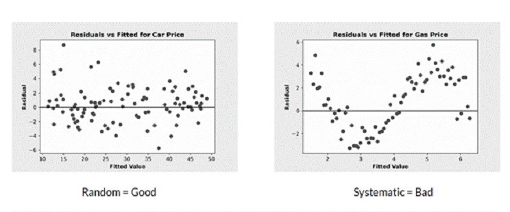
 Another model debugging technique is Residual Analysis. In most cases, this can be used for regression models. Residual Analysis requires measuring the distance between the prediction and the ground truth. In general, whilst measuring the distance between the prediction and the ground truth you want the residuals to follow a random distribution as shown in the figure below. If the residuals follow a pattern, it is usually a sign that your model has to be improved. 

Thus, using a residual plot one would visually inspect the distribution of residuals. IF your model is well trained and has captured the predictive information in the data, then, the residuals should be randomly distributed.

Co-relation between Residuals

Also – Residuals should not be co-related with each other. If you can use one residual to predict another Residual, the, the Residuals are co-related which means that there is some predictive information that is not being c captured. Performing a Durbin-Watson test is also useful for detecting auto-correlation

Durbin-Watson Test

A Durbin-Watson will report a test statistic with a value between 0 and 4, where:

·        A Value of 2 is no correlation

·        0 to <2 is positive correlation

·        >2 to 4 is negative correlation

As a rule of thumb, the test statistic value in the range of 1.5 to 2.5 is relatively normal. 

Durbin Watson Test in Python: https://www.statology.org/durbin-watson-test-python/